4  {peacesciencer} Basics

The {peacesciencer} package was developed by Miller (2022) to help solve a persistent problem in peace science research. Any time a researcher wants to begin a new study, they face the time-consuming task of generating data from scratch and merging in additional relevant data points for analysis. A considerable amount of new computer code either needs to be written to make this happen, or old code, either that written previously by a researcher for a past study or that created by another researcher, must be adapted for a new purpose. The amount of code produced through this process is such that “the contemporary quantitative political scientist is increasingly becoming a computer programmer” (Miller 2022). The cognitive burden this creates is enough to deter many people with a deep interest in studying problems in politics and policy (such as peace and war) from continuing with their research.

The goal behind {peacesciencer} is to remove this critical barrier to doing quantitative research in the realm of conflict. The field of peace science—which is a sub-field of International Relations, which in turn is a sub-field of political science—addresses normatively weighty questions dealing with the causes of war and whether sustainable peace is possible. By limiting some of the friction many peace science researchers run into, it will be possible to produce more research transparently and in such a way that is easy to replicate by others. In this way, {peacesciencer} is consistent with the Data Access and Research Transparency initiative (DA-RT) in the social sciences.

In support of this goal, {peacesciencer} makes it possible “to load data, create data, clean data, analyze data, and present the results of the analysis all within one program” (Miller 2022). The package can’t do all this on its own, but because it works with R, and specifically within the increasingly popular {tidyverse} set of packages, it is possible to complete a research project from start to finish using conflict data generated with {peacesciencer} all with R and in the free-to-use integrated development environment (IDE) provided via RStudio (soon to be Posit Workbench).

How to use the tools in the {peacesciencer} package to create and clean datasets for analysis is a key skill that you’ll develop by practicing the examples laid out in the coming chapters. These skills will lay a foundation for incorporating new datasets not covered under the {peacesciencer} umbrella. By the time you finish, you should be an efficient data analyst with the ability to do insightful peace science research.

Before we get too far ahead of ourselves, we first need to become familiar with the basics of working with {peacesciencer}. The remainder of this chapter is dedicated to summarizing the main kinds of datasets that you can create and how you can merge in a wide variety of additional datasets accessible through {peacesciencer}. Let’s get to it.

4.1 Installing {peacesciencer}

The {peacesciencer} package was created for use in the R programming language, and in particular it’s designed to share a common syntax with the component packages of {tidyverse}. The latter is essentially a meta-package that, once opened, loads a number of packages that are part of the “tidyverse,” which are meant to be used in concert.

To install each package, you’ll need to open an R session in RStudio or Posit Workbench and write the following in your R console:

install.packages(c("tidyverse", "peacesciencer"))

Once they’ve been installed, any time you want to use these packages, you’ll just need to load both in your R session using the library() function, like so:

library(tidyverse)
library(peacesciencer)

You now can start working with the tools in {peacesceincer} to create the kind of data you need for your research.

4.2 How to Create Base Data

As Miller (2022) states, “{peacesciencer} comes with a fully developed suite of built-in functions for generating some of the most widespread forms of peace science data and populating the data with important variables that recur in many quantitative analyses.” These functions fall under two umbrellas, one for creating base data and the other for adding variables of interest.

Any new analysis will start by creating a base dataset. {peacesciencer} provides tools to let you create six different kinds of base data. These vary based on the unit of analysis under study (political leaders, countries, or dyads) and the unit of time (days or years). A summary of these functions is given below:

• create_dyadyears() - Create dyad-years (a dyad is a pair of countries) from state system membership data (either COW or GW)

• create_leaderdays() - Create leader-day data from Archigos

• create_leaderdyadyears() - Create leader-dyad-years data from Archigos

• create_leaderyears() - Create leader-years data from Archigos

• create_statedays() - create state-days data from state system membership data (either COW or GW)

• create_stateyears() - create state-years data from state system membership data (either COW or GW)

These functions will return a base dataset with the desired unit of analysis and at the desired unit of time. For example, if you want the full universe of state-years in the world starting at 1816 to the most recently concluded calendar year, you can use create_stateyears() as your starting place. The function will either base this universe on the Correlates of War (CoW) or Gleditsch-War (GW) state systems, depending on the arguments you provide. For instance, by default, the function returns countries based on the CoW system:

sy_data <- create_stateyears()
glimpse(sy_data)

Rows: 17,316
Columns: 3
$ ccode    <dbl> 2, 2, 2, 2, 2, 2, 2, 2, 2, 2, 2, 2, 2, 2, 2, 2, 2, 2, 2, 2, 2…
$ statenme <chr> "United States of America", "United States of America", "Unit…
$ year     <int> 1816, 1817, 1818, 1819, 1820, 1821, 1822, 1823, 1824, 1825, 1…

In the above code, I told R to create a state-year dataset using the default settings in create_stateyears() and had it save the output as an object called sy_data. I then used glimpse() to report a quick overview of the data. It has three columns: ccode, statenme, and year.¹ The latter two are obvious—they give the name of the country in question and the relevant year it is recorded as being part of the international state system according to CoW. The value of ccode is a numerical code created by CoW to provide a consistent way of referring to specific states.

If we wanted, instead, to create a state-years dataset based on the GW system, we can tell create_stateyears() to do so:

sy_data <- create_stateyears(system = "gw")
glimpse(sy_data)

Rows: 18,811
Columns: 3
$ gwcode    <dbl> 2, 2, 2, 2, 2, 2, 2, 2, 2, 2, 2, 2, 2, 2, 2, 2, 2, 2, 2, 2, …
$ statename <chr> "United States of America", "United States of America", "Uni…
$ year      <int> 1816, 1817, 1818, 1819, 1820, 1821, 1822, 1823, 1824, 1825, …

Notice that the data no longer has a column called ccode. Instead it has a column called gwcode. Notice, too, that the size of the data is not identical to the one produced with the CoW state system. The reason is that CoW and GW have slightly different approaches to classifying whether some political entity counts as a state. I highly recommend reading this discussion of the two different state systems if you want to learn more about each and when one is more appropriate than the other.

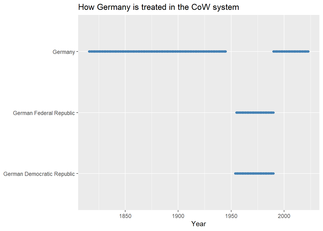
As one example of the differences between these different coding schemes, consider Germany. Dating back to 1816 the territory that would later be organized under the name “Germany” was called Prussia. Once it became Germany, it remained unified until after WWII. During the Cold War it was carved up into the German Federal Republic (to the west) and the German Democratic Republic (to the east). After the Cold War, the two Germanies were unified under the German Federal Republic.

This seems like a straightforward set of events, but when it comes to how we should study Germany over time using data, it creates the need to make a tough choice. Is the Germany of today a continuation of the Germany that existed before the Cold War (before it was divided into two countries), or did the Germany that existed in the lead up to WWII cease to exist and was replaced by the German Federal Republic and the German Democratic Republic, the latter of which was then folded into the German Federal Republic after the Cold War? CoW and GW answer this question in different ways.

Let’s create data based on each system:

cow_sys <- create_stateyears()
gw_sys <- create_stateyears(system = "gw")

Next, let’s filter the data down to all instances of “Germany” in the data and look at which Germanies exist at which points in time according to CoW:

cow_sys |>
  filter(str_detect(statenme, "German")) |>
  ggplot() +
  aes(x = year, y = statenme) +
  geom_point(
    color = "steelblue"
  ) +
  labs(
    x = "Year",
    y = NULL,
    title = "How Germany is treated in the CoW system"
  )

Let’s compare to the GW system:

gw_sys |>
  filter(str_detect(statename, "German")) |>
  ggplot() +
  aes(x = year, y = statename) +
  geom_point(
    color = "steelblue"
  ) +
  labs(
    x = "Year",
    y = NULL,
    title = "How Germany is treated in the GW system"
  )

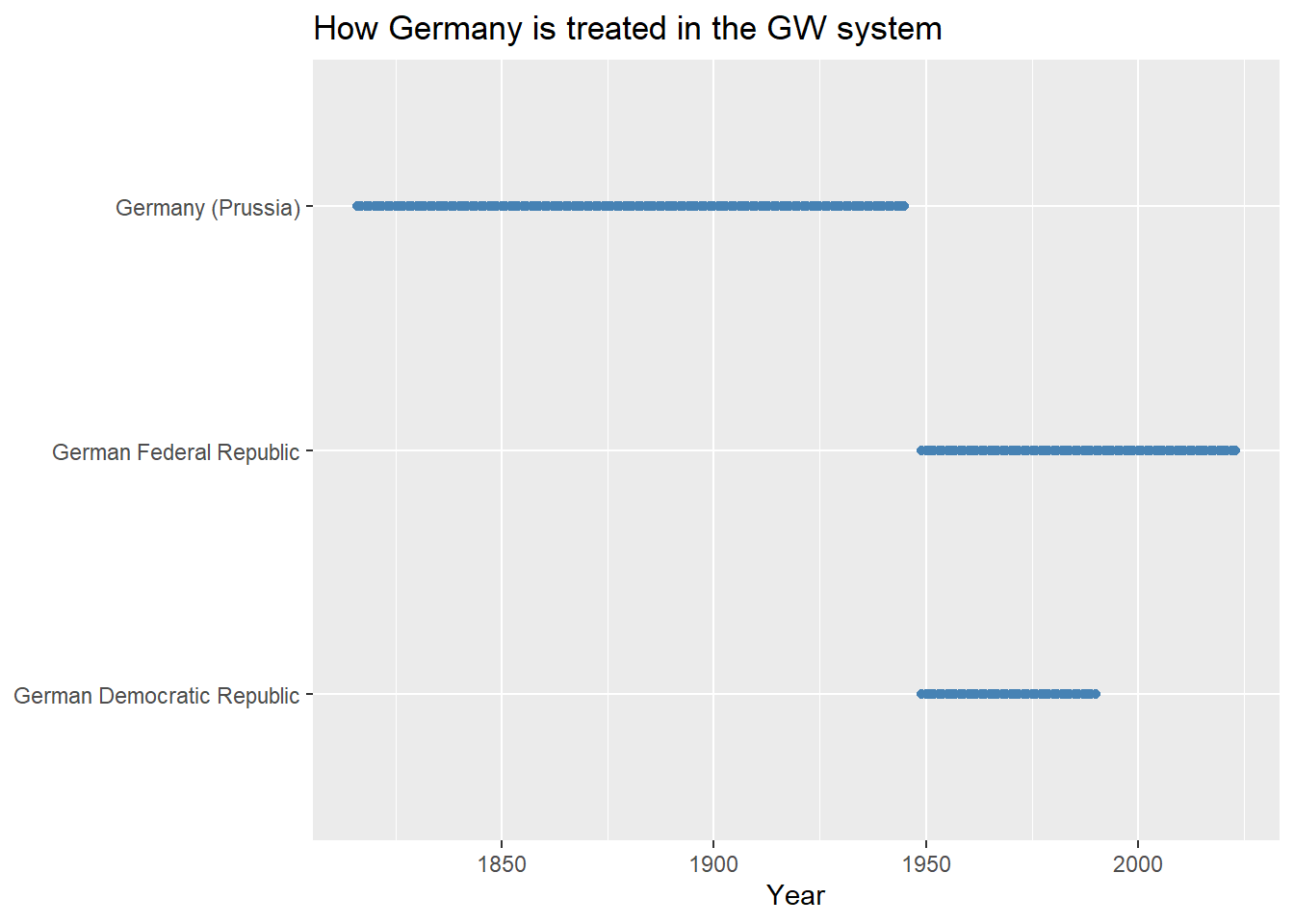
From the above, it’s clear that CoW treats the Germany of today as a return to the unified German state that existed prior to the Cold War. GW, on the other hand, treats the Germany of today as the German Federal Republic (distinct from the Germany that existed prior to the Cold War).

The question of which of these systems is the correct system is the wrong question to ask. The better question to consider is whether one or the other system plays more nicely with the data you’d like to add to the base data. For example, if you want to populate your dataset with CoW data on international or intranational conflicts, you should create your data using the CoW state system. However, if you want to use UCDP/PRIO conflict data (also accessible with {peacesciencer}), you’ll want to use the GW system since this conflict data is based on this state system rather than on CoW’s.

Importantly, if you ever need to start with one system, but need to use data that plays nicely with the other system, you can include the relevant codes for the other system in your data. For example, say we wanted add GW codes to the CoW system data we created. The function add_gwcode_to_cow() let’s us do that:

cow_sys <- cow_sys |>
  add_gwcode_to_cow()

Joining with `by = join_by(ccode, year)`

glimpse(cow_sys)

Rows: 17,316
Columns: 4
$ ccode    <dbl> 2, 2, 2, 2, 2, 2, 2, 2, 2, 2, 2, 2, 2, 2, 2, 2, 2, 2, 2, 2, 2…
$ statenme <chr> "United States of America", "United States of America", "Unit…
$ year     <dbl> 1816, 1817, 1818, 1819, 1820, 1821, 1822, 1823, 1824, 1825, 1…
$ gwcode   <dbl> 2, 2, 2, 2, 2, 2, 2, 2, 2, 2, 2, 2, 2, 2, 2, 2, 2, 2, 2, 2, 2…

The state system is still the CoW system. But, the a new column is added to the data that translates CoW codes to GW codes (the data have both a ccode column and a gwcode column). If we wanted to add CoW codes to the GW system data, we can use a similar function called add_ccode_to_gw().

4.3 Populating your Data with New Variables

Once you’ve created your base data, the next step is to start populating it with variables that you want to study. The {peacesciencer} package has 27 add_*() functions (as of this writing) that let you incorporate data from numerous commonly used datasets by peace science scholars. To get a quick summary of what’s available, you can use the ps_version() function. The below code uses this function and gives it to kbl() to report the results in a tidier looking table:

library(kableExtra)
ps_version() |>
  kbl(
    caption = "Data Available in `{peacesciencer}`"
  )

Data Available in `{peacesciencer}`

category	data	version	bibtexkey
states	Correlates of War State System Membership	2016	cowstates2016
leaders	LEAD	2015	ellisetal2015lead
leaders	Archigos	4.1	goemansetal2009ia
alliance	ATOP	5	leedsetal2002atop
alliance	Correlates of War Formal Alliances	4.1	gibler2009ima
democracy	Polity	2017	marshalletal2017p
democracy	{QuickUDS}	0.2.3	marquez2016qme
democracy	V-Dem	10	coppedgeetal2020vdem
capitals	{peacesciencer}	2020	peacesciencer-package
contiguity	Correlates of War Direct Contiguity	3.2	stinnettetal2002cow
igo	Correlates of War IGOs	3	pevehouseetal2020tow
majors	Correlates of War	2016	cowstates2016
conflict_interstate	Correlates of War Militarized Interstate Disputes	5	palmeretal2021mid5
distance	{Cshapes}	2	schvitz2021mis
capabilities	Correlates of War National Material Capabilities	6	singer1987rcwd
gdp	SDP	2020	andersetal2020bbgb
sdp	SDP	2020	andersetal2020bbgb
population	SDP	2020	andersetal2020bbgb
trade	Correlates of War Trade	4	barbierietal2009td
conflict_intrastate	Correlates of War Intra-State War	4.1	dixonsarkees2016giw
conflict_interstate	Correlates of War Inter-State War	4	sarkeeswayman2010rw
fractionalization	CREG	2012	nardulli2012creg
polarization	CREG	2012	nardulli2012creg
conflict_interstate	Gibler-Miller-Little (GML)	2.2.1	gibleretal2016amid
states	Gleditsch-Ward	2017	gledtischward1999rlis
leaders	Leader Willingness to Use Force	2020	cartersmith2020fml
terrain	Ruggedness	2012	nunnpuga2012r
terrain	% Mountainous	2014	giblermiller2014etts
rivalries	Thompson and Dreyer	2012	thompsondreyer2012hir
conflict_intrastate	UCDP Armed Conflicts	20.1	gleditschetal2002ac
conflict_intrastate	UCDP Onsets	19.1	pettersson2019ov
dyadic_similarity	FPSIM	2	haege2011cc

For each one of the above datasets, there is a relevant add_*() function that will populate a base dataset.

For example, let’s make a dataset that has for state-years information about the occurrence of civil wars using the UCDP/PRIO measure of civil wars and quality of democracy.

## start with GW system data (subset years to 1946-2014)
gw_data <- create_stateyears(
  system = "gw",
  subset_years = 1946:2014
)

## add conflict and democracy data
gw_data <- gw_data |>
  add_ucdp_acd() |>
  add_democracy()

Joining with `by = join_by(gwcode, year)`
Joining with `by = join_by(gwcode, year)`

## take a glimpse
glimpse(gw_data)

Rows: 9,620
Columns: 10
$ gwcode        <dbl> 2, 2, 2, 2, 2, 2, 2, 2, 2, 2, 2, 2, 2, 2, 2, 2, 2, 2, 2,…
$ statename     <chr> "United States of America", "United States of America", …
$ year          <dbl> 1946, 1947, 1948, 1949, 1950, 1951, 1952, 1953, 1954, 19…
$ ucdpongoing   <dbl> 0, 0, 0, 0, 1, 0, 0, 0, 0, 0, 0, 0, 0, 0, 0, 0, 0, 0, 0,…
$ ucdponset     <dbl> 0, 0, 0, 0, 1, 0, 0, 0, 0, 0, 0, 0, 0, 0, 0, 0, 0, 0, 0,…
$ maxintensity  <dbl> NA, NA, NA, NA, 1, NA, NA, NA, NA, NA, NA, NA, NA, NA, N…
$ conflict_ids  <chr> NA, NA, NA, NA, "238", NA, NA, NA, NA, NA, NA, NA, NA, N…
$ v2x_polyarchy <dbl> 0.605, 0.587, 0.599, 0.599, 0.587, 0.602, 0.601, 0.594, …
$ polity2       <dbl> 10, 10, 10, 10, 10, 10, 10, 10, 10, 10, 10, 10, 10, 10, …
$ xm_qudsest    <dbl> 1.259180, 1.259180, 1.252190, 1.252190, 1.270106, 1.2594…

A question that we could ask with this data is whether or not democracy has any correlation with the likelihood of civil war? The below code tells R to create a figure showing quality of democracy (the v2x_polyarchy measure from V-Dem) on the x-axis and the UCDP measure of civil war onset on the y-axis. It uses a simple logistic regression model to summarize how quality of democracy is related to the probability that a country fights a civil war.

ggplot(gw_data) +
  aes(x = v2x_polyarchy, y = ucdponset) +
  stat_smooth(
    method = "glm",
    method.args = list(family = binomial)
  ) +
  labs(
    x = "Quality of Democracy",
    y = "Probability of Civil War",
    title = "Civil war onset (UCDP) and democracy"
  )

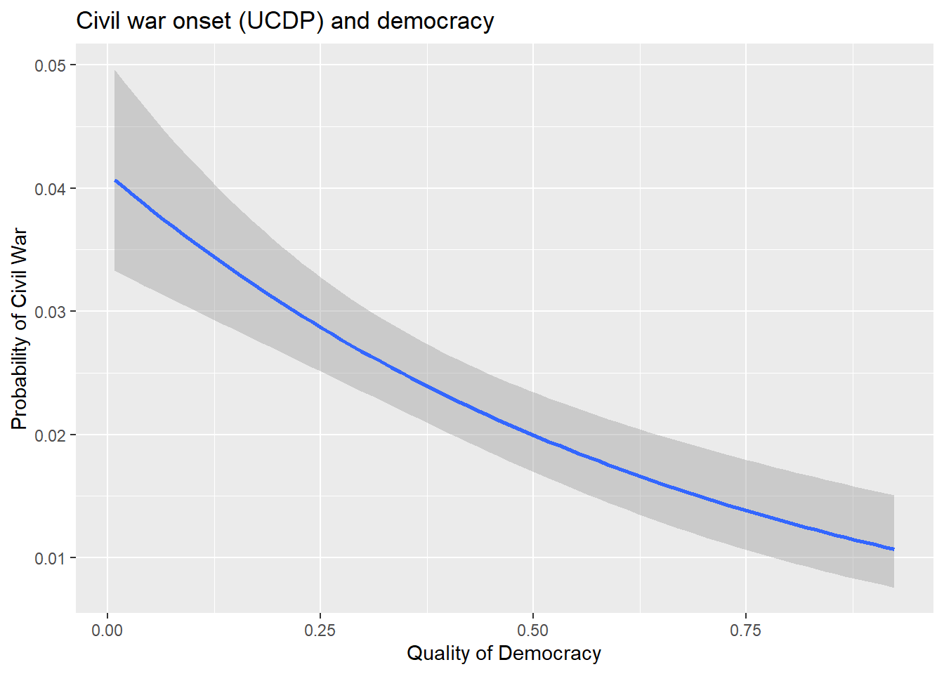
We’ll cover the usefulness of factors such as democracy for explaining variation in conflict in later chapters. For now, we’ll just note that the correlation between democracy and civil war is pretty strong and negative. Civil wars are just less likely to occur in democracies relative to non-democracies.

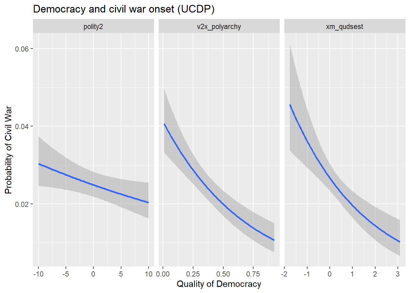
Of course, we could have used a different measure of democracy. It’s possible that the one we used is biased, offering a misleading picture of the relationship between democracy and civil war. The add_democracy() function adds three measures of democracy to the data that we might want to consider:

• v2x_polyarchy - the level of democracy on a 0 to 1 scale measured by the Varieties of Democracy (V-Dem) project

• polity2 - the level of democracy on a -10 to 10 scale measured by the Polity project

• xm_qudsests - the level of democracy in standard deviation units based on Xavier Marquez’s QuickUDS extensions/estimates based on the Unified Democracy Scores project

Each of these measures of democracy are based on some overlapping, but also diverging criteria. The below code tells R to report a similar figure to the one produced above, but this time it tells it to produce three smaller figures side-by-side for each measure. Based on the results, it’s pretty clear that both the UDS and V-Dem measures show a strong negative correlation with civil war. The Polity measure has a negative relationship with conflict as well, but its magnitude is somewhat attenuated.

gw_data |>
  pivot_longer(
    v2x_polyarchy:xm_qudsest
  ) |>
  ggplot() +
  aes(x = value, y = ucdponset) +
  stat_smooth(
    method = "glm",
    method.args = list(family = binomial)
  ) +
  facet_wrap(~ name, scales = "free_x") +
  labs(
    x = "Quality of Democracy",
    y = "Probability of Civil War",
    title = "Democracy and civil war onset (UCDP)"
  )

The {peacesciencer} package provides the ability to perform very detailed analyses. One of the main examples that Miller (2022) discusses is a replication of the “dangerous dyads” analysis by Bremer (1992) which incorporates several datasets to study the factors that make a pair of countries especially likely to engage in a militarized dispute.² The below code creates a dataset that lets us replicate Bremer’s analysis.

# create base data, and pipe (|>) to next function
create_dyadyears(directed = FALSE, subset_years = c(1816:2010)) |>
  # subset data to politically relevant dyads (PRDs), pipe to next function
  filter_prd() |>
  # add conflict information from GML-MID data, pipe to next function
  add_gml_mids(keep = NULL) |>
  # add peace years ("spells"), pipe to next function
  add_spells() |>
  # add capabilities data, pipe to next function
  add_nmc() |>
  # add some estimates about democracy for each state, pipe to next function
  add_democracy() |>
  # add information about alliance commitments in dyad-year
  add_cow_alliance() |>
  # finish with information about population and GDP/SDP
  # and then assign to object, called, minimally, 'Data'
  add_sdp_gdp() -> Data

Joining with `by = join_by(ccode1, ccode2, year)`
Joining with `by = join_by(ccode1, ccode2, year)`
Dyadic data are non-directed and initiation variables make no sense in this
context.
Joining with `by = join_by(ccode1, ccode2, year)`
add_gml_mids() IMPORTANT MESSAGE: By default, this function whittles
dispute-year data into dyad-year data by first selecting on unique onsets.
Thereafter, where duplicates remain, it whittles dispute-year data into
dyad-year data in the following order: 1) retaining highest `fatality`, 2)
retaining highest `hostlev`, 3) retaining highest estimated `mindur`, 4)
retaining highest estimated `maxdur`, 5) retaining reciprocated over
non-reciprocated observations, 6) retaining the observation with the lowest
start month, and, where duplicates still remained (and they don't), 7) forcibly
dropping all duplicates for observations that are otherwise very similar. See:
http://svmiller.com/peacesciencer/articles/coerce-dispute-year-dyad-year.html

Warning in xtfrm.data.frame(x): cannot xtfrm data frames

Joining with `by = join_by(orig_order)`
Joining with `by = join_by(ccode1, ccode2, year)`

glimpse(Data)

Rows: 112,282
Columns: 42
$ ccode1          <dbl> 2, 2, 2, 2, 2, 2, 2, 2, 2, 2, 2, 2, 2, 2, 2, 2, 2, 2, …
$ ccode2          <dbl> 20, 20, 20, 20, 20, 20, 20, 20, 20, 20, 20, 20, 20, 20…
$ year            <dbl> 1920, 1921, 1922, 1923, 1924, 1925, 1926, 1927, 1928, …
$ conttype        <dbl> 1, 1, 1, 1, 1, 1, 1, 1, 1, 1, 1, 1, 1, 1, 1, 1, 1, 1, …
$ cowmaj1         <dbl> 1, 1, 1, 1, 1, 1, 1, 1, 1, 1, 1, 1, 1, 1, 1, 1, 1, 1, …
$ cowmaj2         <dbl> 0, 0, 0, 0, 0, 0, 0, 0, 0, 0, 0, 0, 0, 0, 0, 0, 0, 0, …
$ prd             <dbl> 1, 1, 1, 1, 1, 1, 1, 1, 1, 1, 1, 1, 1, 1, 1, 1, 1, 1, …
$ gmlmidonset     <dbl> 0, 0, 0, 0, 0, 0, 0, 0, 0, 0, 0, 0, 0, 0, 0, 0, 0, 0, …
$ gmlmidongoing   <dbl> 0, 0, 0, 0, 0, 0, 0, 0, 0, 0, 0, 0, 0, 0, 0, 0, 0, 0, …
$ gmlmidspell     <dbl> 0, 1, 2, 3, 4, 5, 6, 7, 8, 9, 10, 11, 12, 13, 14, 15, …
$ milex1          <dbl> 1657118, 1116342, 860853, 678256, 570142, 589706, 5580…
$ milper1         <dbl> 343, 387, 270, 247, 261, 252, 247, 249, 251, 255, 256,…
$ irst1           <dbl> 42809, 20101, 36173, 45665, 38540, 46122, 49069, 45656…
$ pec1            <dbl> 743808, 622541, 641311, 834889, 762070, 790029, 852304…
$ tpop1           <dbl> 106461, 108538, 110049, 111947, 114109, 115829, 117397…
$ upop1           <dbl> 27428, 28210, 29013, 29840, 30690, 31565, 32464, 33389…
$ cinc1           <dbl> 0.2895664, 0.2532295, 0.2555951, 0.2720777, 0.2535910,…
$ milex2          <dbl> 10755, 10209, 10028, 13316, 12824, 12984, 13936, 16745…
$ milper2         <dbl> 4, 4, 4, 4, 4, 4, 4, 4, 5, 4, 5, 6, 5, 5, 5, 4, 6, 6, …
$ irst2           <dbl> 1118, 678, 494, 899, 661, 765, 789, 922, 1255, 1400, 1…
$ pec2            <dbl> 31979, 30630, 26533, 35626, 29947, 29242, 33207, 36491…
$ tpop2           <dbl> 8556, 8788, 8919, 9010, 9143, 9294, 9451, 9637, 9835, …
$ upop2           <dbl> 1598, 1659, 1708, 1760, 1822, 1893, 1971, 2054, 2119, …
$ cinc2           <dbl> 0.010128360, 0.010542275, 0.008407704, 0.009860509, 0.…
$ v2x_polyarchy1  <dbl> 0.446, 0.509, 0.510, 0.516, 0.514, 0.505, 0.511, 0.530…
$ polity21        <dbl> 10, 10, 10, 10, 10, 10, 10, 10, 10, 10, 10, 10, 10, 10…
$ xm_qudsest1     <dbl> 1.185981, 1.185981, 1.192117, 1.192117, 1.201639, 1.20…
$ v2x_polyarchy2  <dbl> 0.442, 0.576, 0.622, 0.622, 0.622, 0.622, 0.661, 0.672…
$ polity22        <dbl> 9, 10, 10, 10, 10, 10, 10, 10, 10, 10, 10, 10, 10, 10,…
$ xm_qudsest2     <dbl> 0.9818035, 1.3082951, 1.3094862, 1.3094862, 1.3094862,…
$ cow_defense     <dbl> 0, 0, 0, 0, 0, 0, 0, 0, 0, 0, 0, 0, 0, 0, 0, 0, 0, 0, …
$ cow_neutral     <dbl> 0, 0, 0, 0, 0, 0, 0, 0, 0, 0, 0, 0, 0, 0, 0, 0, 0, 0, …
$ cow_nonagg      <dbl> 0, 0, 0, 0, 0, 0, 0, 0, 0, 0, 0, 0, 0, 0, 0, 0, 0, 0, …
$ cow_entente     <dbl> 0, 0, 0, 0, 0, 0, 0, 0, 0, 0, 0, 0, 0, 0, 0, 0, 0, 0, …
$ wbgdp2011est1   <dbl> 27.641, 27.648, 27.698, 27.766, 27.817, 27.855, 27.889…
$ wbpopest1       <dbl> 18.449, 18.472, 18.488, 18.508, 18.519, 18.534, 18.546…
$ sdpest1         <dbl> 27.523, 27.527, 27.582, 27.656, 27.711, 27.751, 27.788…
$ wbgdppc2011est1 <dbl> 9.193, 9.176, 9.210, 9.259, 9.298, 9.321, 9.343, 9.346…
$ wbgdp2011est2   <dbl> 24.835, 24.819, 24.848, 24.884, 24.946, 25.008, 25.051…
$ wbpopest2       <dbl> 15.946, 15.962, 15.976, 15.988, 16.006, 16.020, 16.038…
$ sdpest2         <dbl> 24.672, 24.650, 24.682, 24.722, 24.791, 24.860, 24.908…
$ wbgdppc2011est2 <dbl> 8.890, 8.857, 8.872, 8.897, 8.940, 8.988, 9.014, 9.044…

The above code creates a non-directed dyad-years dataset as the base. “Non-directed” just means that for a given dyad (a pair of countries) in the international system, if a country is on side 1 in the pair, it doesn’t appear as side 2 for the same pair again (e.g., there are no repeats). Just to quickly highlight the difference, consider the following datasets which give either the universe of directed dyads or the universe of non-directed dyads in the year 2023:

## create directed dyad data for 2023
dd_23 <- create_dyadyears(subset_years = 2023)

Joining with `by = join_by(ccode1, ccode2, year)`

## create non-directed dyad data for 2023
nd_23 <- create_dyadyears(directed = F, subset_years = 2023)

Joining with `by = join_by(ccode1, ccode2, year)`

Since one includes directed dyads, it should be larger than the one with non-directed dyads:

## check number of rows
nrow(dd_23) > nrow(nd_23)

[1] TRUE

Sure enough, the directed dyad data is bigger. In fact, it’s double the size of the other:

## check that nrow(dd_23) == 2 * nrow(nd_23) == TRUE
nrow(dd_23) == 2 * nrow(nd_23)

[1] TRUE

The reason is that one repeats dyads while the other does not. Let’s look at the US-Canada dyad in each dataset to illustrate. The below code creates a table of the US-Canada pairs for 2023 in the directed dyad dataset. Notice that there are two. In one, the US is on side 1 and Canada is on side 2. In the other, the US is on side 2 while Canada is on side 1.

## US code is 2 and CAN code is 20
dd_23 |>
  filter(
    ccode1 %in% c(2, 20),
    ccode2 %in% c(2, 20)
  ) |>
  kbl(
    caption = "Directed Dyad Data (US and Canada)"
  )

Directed Dyad Data (US and Canada)

ccode1	ccode2	year
2	20	2023
20	2	2023

Let’s take a look at the non-directed dyad. The table produced below shows every instance of the US-Canada dyad for 2023 in the non-directed dyad data. As you can see, there is only one instance. The US appears on side 1 and Canada on side 2, and that’s it.

nd_23 |>
  filter(
    ccode1 %in% c(2, 20),
    ccode2 %in% c(2, 20)
  ) |>
  kbl(
    caption = "Non-Directed Dyad Data (US and Canada)"
  )

Non-Directed Dyad Data (US and Canada)

ccode1	ccode2	year
2	20	2023

Just like the case with choosing between state systems (CoW vs. GW), there is no universally correct choice between directed and non-directed dyad data. It depends on what data you want to use and your research question. In the case of the “dangerous dyads” study by Bremer (1992), non-directed dyads are the way to go. The purpose of the study was to look at the correlates of conflict initiation between a pair of countries, but the focus isn’t on the factors that make one of the countries in the pair more likely to initiate a conflict versus the other. If the goal was, instead, to study why one country is more apt to start a fight than another, then a directed dyad dataset would make sense.

Okay, let’s get back to the replication of Bremer (1992)…

Once the base data is created using create_dyadyears(), the filter_prd() function subsets the data down to “politically relevant dyads.” You can read more about what this means by writing ?filter_prd() in the R console. The gist is that it uses information about whether a pair of countries is contiguous (share a border) or if one of the countries is a major power to determine whether it makes sense to study conflict between a pair of countries. The idea is that major powers have the capacity to fight wars over longer distances, so if one of the countries in a pair is a major power, it’s probably feasible for the two to fight. Outside of major powers, most other countries probably are unlikely to fight unless they border each other or are at least geographically proximate since they lack the capacity to fight a war at a greater distance. If a dyad is not politically relevant according to these criteria, filter_prd() drops that dyad from the dataset.

From here, the dataset is populated with information about whether a pair of countries engages in a militarized interstate dispute (MID) based on the Douglas M. Gibler, Miller, and Little (2016) measure. It also adds information about spells of peace, military capabilities, democracy, alliances, and economic data. With it, it is possible to replicate the “dangerous dyads” analysis by Bremer (1992). First, the data need to be recoded a bit to create the variables Bremer used:

Data |>
  # Create dummies for contiguity and major power dyads
  mutate(landcontig = ifelse(conttype == 1, 1, 0)) |>
  mutate(cowmajdyad = ifelse(cowmaj1 == 1 | cowmaj2 == 1, 1, 0)) |>
  # Create estimate of militarization as milper/tpop
  # Then make a weak-link
  mutate(milit1 = milper1/tpop1,
         milit2 = milper2/tpop2,
         minmilit = ifelse(milit1 > milit2,
                           milit2, milit1)) |>
  # Create CINC proportion (lower over higher)
  mutate(cincprop = ifelse(cinc1 > cinc2,
                           cinc2/cinc1, cinc1/cinc2)) |>
  # Create weak-link specification using Quick UDS data
  mutate(mindemest = ifelse(xm_qudsest1 > xm_qudsest2,
                            xm_qudsest2, xm_qudsest1)) |>
  # Create "weak-link" measure of jointly advanced economies
  mutate(minwbgdppc = ifelse(wbgdppc2011est1 > wbgdppc2011est2,
                             wbgdppc2011est2, wbgdppc2011est1)) -> Data

Now, with the updated data, we can estimate a model of conflict onset (using logistic regression) given a number of predictors. The model also includes a cubic peace spells trend. Logistic regression models, (or just logit models) are the standard way that conflict scholars study why conflicts start. The reason is that logit models are ideally suited to studying variation in binary outcomes. Conflict onset is an example of binary data because a conflict either takes place (represented by a 1) or it doesn’t (represented by a 0).

Such outcomes can be studied using a standard linear regression model, but sometimes this approach leads to predictions that are either greater than 1 or less than 0. We call this 0-1 range the unit interval, which reflects the bounds for values an outcome can take. Think of it this way, if an outcome is binary then statistically speaking it can either occur (1) or not occur (0) with some probability \(p\). A probability inherently cannot be greater than 1 or less than 0. When we’re dealing with binary outcomes, the goal with a regression analysis is to model the probability that an event occurs given a set of explanatory variables. A logit model is designed with this in mind. Rather than show you with equations, it’ll be better to show you with some pictures.

In the below code I told R to simulate some binary data \(y\) that is correlated with a variable called \(x\). I then told R to estimate a standard linear regression model of how values of \(x\) determine the probability of \(y\) and also a logit model. Notice the difference in the slopes. The linear model is, as you would guess, linear. But the logit model captures the relationship between \(x\) and \(y\) as an s-shaped curve. This s-shape is such that the logit model will never report a probability for an outcome that is greater than 1 or less than 0. In contrast, there’s nothing to stop the linear model from reporting a value for \(y\) outside these bounds. This is why most conflict research is done using logit.

library(geomtextpath)
set.seed(111)
sim_data <- tibble(
  x = 1:100,
  y = rbinom(
    n = length(x),
    size = 1,
    prob = x / max(x)
  )
)
ggplot(sim_data) +
  aes(x = x, y = y) +
  geom_textsmooth(
    method = "lm",
    label = "Linear Model",
    color = "red3",
    hjust = 0.8
  ) +
  geom_textsmooth(
    method = "glm",
    method.args = list(family = binomial),
    label = "Logit Model",
    color = "steelblue",
    hjust = 0.2
  ) +
  scale_y_continuous(
    breaks = 0:1
  ) +
  geom_hline(
    yintercept = 0:1,
    linetype = 2
  ) +
  labs(
    title = "Linear vs. logit model for binary outcomes"
  )

`geom_smooth()` using formula = 'y ~ x'
`geom_smooth()` using formula = 'y ~ x'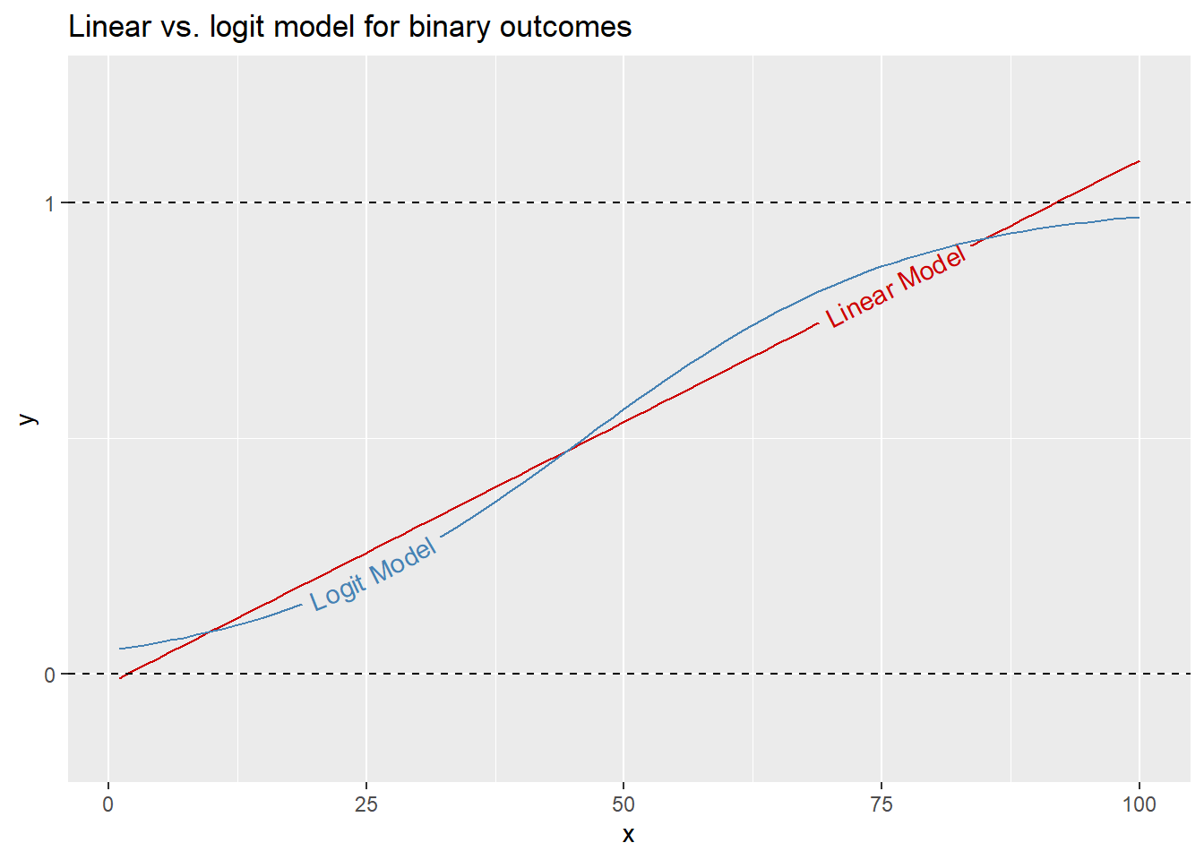

Back to the replication of Bremer (1992), the below code tells R to estimate a logit model of MID onset using a number of different explanatory variables. It then tells R to report the output in a table. The table reports for each variable in the logistic regression model the estimated coefficient (slope) along with its standard error, z-statistic, and p-value. Think of this slope as determining how severe the s-shaped line is that represents the probability of MID onset and whether it’s increasing or decreasing. For this slope, we usually say that when the p-value is less than 0.05 an estimate is “statistically significant,” meaning we can reject the null hypothesis that the true slope coefficient is zero. According to the below results, all of the variables included in the model have a statistically significant relationship with conflict onset between a pair of countries.

## estimate the model
model <- glm(
  gmlmidonset ~ landcontig + cincprop + cowmajdyad + cow_defense +
               mindemest + minwbgdppc + minmilit +
               gmlmidspell + I(gmlmidspell^2) + I(gmlmidspell^3),
  data = Data,
  family = binomial
)

## report the regression results with kbl()
broom::tidy(model) |>
  kbl(
    caption = "Dangerous Dyads Analysis",
    digits = 3
  )

Dangerous Dyads Analysis

term	estimate	std.error	statistic	p.value
(Intercept)	-4.035	0.141	-28.684	0.000
landcontig	1.062	0.057	18.709	0.000
cincprop	1.022	0.082	12.509	0.000
cowmajdyad	0.144	0.057	2.512	0.012
cow_defense	-0.119	0.058	-2.044	0.041
mindemest	-0.291	0.031	-9.509	0.000
minwbgdppc	0.090	0.016	5.720	0.000
minmilit	26.641	2.365	11.262	0.000
gmlmidspell	-0.147	0.005	-29.007	0.000
I(gmlmidspell^2)	0.002	0.000	18.360	0.000
I(gmlmidspell^3)	0.000	0.000	-13.004	0.000

Now, these slope values are somewhat hard to interpret. The way a logit model creates an s-shaped relationship between an explanatory variable and a binary outcome is by transforming the data such that it models the natural log of the odds that an event occurs. The slope values therefore tell us how much the logged odds of an event change per a unit change in the explanatory variable. Most people have a hard time knowing exactly what this means, so it’s usually better to report “marginal effects” instead. These translate logistic regression estimates into probabilities, which most people can understand.

The below code replicates the above, but instead uses the logitmfx() function from the {mfx} R package to estimate the logit model. I like using this for performing logistic regression because the reported estimates are marginal effects (the estimate indicates the change in the probability of the outcome per a change in an explanatory variable). I also like that I can tell the function I want robust standard errors and whether they should be clustered. For most research using observational data (that includes just about all of conflict research), making robust, and sometimes clustered, statistical inferences helps us avoid drawing overly optimistic conclusions about relationships between explanatory variables and an outcome. So, in the case of studying “dangerous dyads,” it’s probably wise to use robust standard errors that are clustered by dyads.

## use {mfx} package to get marginal effects
library(mfx)

## estimate the model
model <- logitmfx(
  gmlmidonset ~ landcontig + cincprop + cowmajdyad + cow_defense +
               mindemest + minwbgdppc + minmilit +
               gmlmidspell + I(gmlmidspell^2) + I(gmlmidspell^3),
  data = Data |> mutate(dyad = paste0(ccode1, ccode2)),
  robust = T,
  clustervar1 = "dyad"
)

## report the regression results with kbl()
broom::tidy(model) |>
  dplyr::select(-atmean) |>
  kbl(
    caption = "Dangerous Dyads Analysis",
    digits = 3
  )

Dangerous Dyads Analysis

term	estimate	std.error	statistic	p.value
landcontig	0.017	0.002	7.883	0.000
cincprop	0.012	0.002	5.500	0.000
cowmajdyad	0.002	0.001	1.468	0.142
cow_defense	-0.001	0.001	-1.280	0.201
mindemest	-0.003	0.001	-6.683	0.000
minwbgdppc	0.001	0.000	3.590	0.000
minmilit	0.308	0.041	7.492	0.000
gmlmidspell	-0.002	0.000	-14.632	0.000
I(gmlmidspell^2)	0.000	0.000	8.544	0.000
I(gmlmidspell^3)	0.000	0.000	-5.513	0.000

The above results are slightly different from those we got using glm(). First, two of the explanatory variables in the model fall short of statistical significance (cowmajdyad and cow_defense). Second, the value under the “estimate” column is now the change in the probability of MID onset given a change in an explanatory variable. For example, the estimate for minmilit, which is a measure of the minimum per capita military expenditures between a pair of countries, is 0.308. This means that for each additional per capita dollar spent on its military by the cheaper spender between two countries, the probability of MID onset increases by 0.308. That’s a large difference. If you multiply it by 100 you get a percent likelihood. Say there’s a 3% baseline likelihood of a MID between a pair of countries. If the weaker military spender between the two increases its military expenditures by 1 dollar for each of its citizens, the likelihood of MID onset between the pair of countries will increase to about 34%. Now, if you’re thinking to yourself “that’s a massive effect for such a small change in spending,” consider that if a country has a population of 50 million, a 1 dollar per capita increase in military spending is equivalent to an absolute increase in spending by 50 million dollars. For many countries, that’s a relatively sizable escalation in military spending.

4.4 Limitations of {peacesciencer}

{peacesciencer} is an incredibly versatile package. It provides researchers with the ability to perform a wide variety of analyses using conflict data and a rich set of covariates that are frequently used by peace scientists. However, the package is not the end-all-be-all for data-driven conflict research. The primary advantage of using the tools in {peacesciencer} is the ability to reliably construct several different base datasets, thus ensuring a transparent and reliable means of constructing the universe of cases you’d like to study. An additional advantage is the ability to populate this dataset with commonly used variables that would otherwise require going to numerous different databases, downloading and cleaning the data from scratch, and then cross-walking and merging the data. Having done all of this myself, I know just how verbose and complicated the code necessary to do this can be—not to mention how time consuming the overall process becomes. All this extra code and time creates space for small errors to snowball into major ones. Therefore, for many of the research questions conflict scholars seek to answer, using {peacesciencer} as a starting point provides obvious benefits.

Nonetheless, the package does not include every possible variable that might be of interest to a researcher. Many new and interesting datasets are created every year. One that we’ll talk about is the Militarized Interstate Events (MIE) dataset that was just introduced last year (Douglas M. Gibler and Miller 2023). To incorporate these datasets we need to make use of some additional tools and packages. This is the subject of the next chapter.

Bremer, Stuart A. 1992. “Dangerous Dyads: Conditions Affecting the Likelihood of Interstate War, 1816-1965.” Journal of Conflict Resolution 36 (2): 309–41.

Gibler, Douglas M., Steven V. Miller, and Erin K. Little. 2016. “An Analysis of the Militarized Interstate Dispute (MID) Dataset, 1816-2001.” International Studies Quarterly 60 (4): 719–30.

Gibler, Douglas M, and Steven V Miller. 2023. “The Militarized Interstate Events (MIE) Dataset, 1816–2014.” Conflict Management and Peace Science, 07388942231182674.

Miller, Steven V. 2022. “\(\{\)Peacesciencer\(\}\): An r Package for Quantitative Peace Science Research.” Conflict Management and Peace Science 39 (6): 755–79.

---

1. The statenme column is actually a typo that made its way into the package. It should be statename (with the “a” included in “name”).

2. The code used to replicate this analysis is adapted from Miller’s analysis which can be found here: https://svmiller.com/peacesciencer/.