5  Cross-walking and Merging New Data

In the previous chapter (Chapter 4) I introduced some of the basics of working with {peacesciencer}. The philosophy behind the package is simple. Reliably and transparently create a base dataset of the universe of cases and time frame that you’d like to study, then populate this dataset with variables of interest. You can choose to look at countries or dyads (pairs of countries), or you can look at country leaders or leader-dyads. You can populate your base data with variables from over thirty different datasets. Your options range from variables related to international wars or military actions short of war and civil wars, and from variables ranging from democracy and economic development to leader experience and willingness to use force.

There will be opportunities to explore a variety of base datasets and combinations of variables in the coming chapters. But before we get there, I want to cover ways that you can incorporate variables from data sources not included with {peacesciencer}. This package is an amazing resource, but it does not give you access to every dataset that you might be interested in. In this chapter, I introduce helpful tools for cross-walking and merging external datasets with {peacesciencer} constructed data.

5.1 What is cross-walking?

The term cross-walking evokes scenes of busy city streets with dense streams of pedestrians moving in unison in Times Square. In data science, the term refers to the process of prepping two or more datasets before trying to combine (merge) them into one. This involves creating common identifiers for observations across datasets so that rows in one can be reliably matched to rows in another. The {peacesciencer} package performs cross-walking for you under the hood most of the time, but in some cases you have to make some changes to a dataset to populate your base data with certain variables.

A good example of this is merging in UCDP/PRIO armed conflict data to a base dataset constructed using the Correlates of War (CoW) state system. The below code tells R to create data using the CoW state system for the years 1946 to 2007. It then tries to merge in UCDP/PRIO data on armed conflicts.

## packages
library(tidyverse)
library(peacesciencer)

## create CoW state system data (county-years)
data <- create_stateyears(subset_years = 1946:2007)

## add UCDP data
data <- data |>
  add_ucdp_acd()

Now, if you ran this code, you’d get the following error when you try to use add_ucdp_acd():

Error in add_ucdp_acd(data) : 
  add_ucdp_acd() merges on the Gleditsch-Ward code (gwcode), which your data don't have right now.

The UCDP/PRIO armed conflict data was constructed using the Gleditsch-Ward (GW) state system; not the CoW state system. That doesn’t mean that we can’t populate our CoW state system dataset with UCDP data. We just need to cross-walk the datasets first. Like I discussed in the previous chapter, we can use some additional {peacesciencer} functions to add country codes from either the CoW state system to a dataset constructed with the GW system, or vice versa. In this case, we just need to use the function add_gwcode_to_cow() to include a column of GW codes in the base dataset we constructed. Then we’ll be able to add the UCDP conflict data.

data <- data |>
  ## cross-walk 
  add_gwcode_to_cow() |>
  ## merge in UCDP conflict data
  add_ucdp_acd()

Joining with `by = join_by(ccode, year)`
Joining with `by = join_by(year, gwcode)`

If we take a glimpse at the data, we can confirm that our base CoW dataset has been populated successfully with the variables from the UCDP armed conflict dataset.

glimpse(data)

Rows: 8,766
Columns: 8
$ ccode        <dbl> 2, 2, 2, 2, 2, 2, 2, 2, 2, 2, 2, 2, 2, 2, 2, 2, 2, 2, 2, …
$ statenme     <chr> "United States of America", "United States of America", "…
$ year         <dbl> 1946, 1947, 1948, 1949, 1950, 1951, 1952, 1953, 1954, 195…
$ gwcode       <dbl> 2, 2, 2, 2, 2, 2, 2, 2, 2, 2, 2, 2, 2, 2, 2, 2, 2, 2, 2, …
$ ucdpongoing  <dbl> 0, 0, 0, 0, 1, 0, 0, 0, 0, 0, 0, 0, 0, 0, 0, 0, 0, 0, 0, …
$ ucdponset    <dbl> 0, 0, 0, 0, 1, 0, 0, 0, 0, 0, 0, 0, 0, 0, 0, 0, 0, 0, 0, …
$ maxintensity <dbl> NA, NA, NA, NA, 1, NA, NA, NA, NA, NA, NA, NA, NA, NA, NA…
$ conflict_ids <chr> NA, NA, NA, NA, "238", NA, NA, NA, NA, NA, NA, NA, NA, NA…

5.2 Cross-walking with {countrycode}

Cross-walking in the context of {peacesciencer} is easy. The task is harder when we want to populate our base data with variables from other data sources. While {peacesciencer} makes it possible to work with two different state systems and their relevant coding schemes, there are way more than two coding systems for countries, and many datasets out there use a coding system other than CoW or GW. In fact, some data sources don’t use a coding system at all. They just use country names, which creates its own set of problems for merging datasets. Even for a country as prominent as the US, this can be an issue. Some data sources use “United States” while others use “United States of America.” Some will use abbreviations—either “US” or “USA” or “U.S.” or “U.S.A.”

This can create headaches for cross-walking datasets for obvious reasons. Thankfully, Arel-Bundock, Enevoldsen, and Yetman (2018) have created an R package that addresses this problem. It’s called {countrycode}, and its workhorse function countrycode() can convert 40+ different coding schemes and 600+ variants of country name spellings to and from one to another. When I first discovered this package, it was a lifesaver. Thankfully, it’s easy to use.

Consider the example below. The {peacesciencer} package isn’t the only R package for accessing data sources. There’s an entire ecosystem of such packages that let users access data from a wide range of databases and for a diverse set of research purposes. One of these packages is {pwt10} which gives R users access to versions 10.0 and 10.01 of the Penn World Table (more about the package here: https://cran.r-project.org/web/packages/pwt10/pwt10.pdf). This dataset was created by a group of economists for studying various measures of income, economic output, input, and productivity for 183 countries from 1950 to 2019. One variable that it contains that might be of interest for studying UCDP armed conflict data is employment. Does the employment rate have anything to do with the likelihood of civil war?

The below code opens the {pwt10} package (if you don’t have it, you can install it by writing install.packages("pwt10") in the R console). It then opens {countrycode} (which you can also install by writing install.packages("countrycode")). Once the package is open, it pipes the data into the mutate() function from the {dplyr} package, which is part of the {tidyverse}. As the name implies, mutate() lets you change or update features of a dataset, either by adding new variables or modifying existing ones. Below, I tell mutate() that I want to add a new column to the Penn World Table dataset called ccode, and using countrycode() I provide instructions for what values to populate this column with. In particular, I tell countrycode() that I want it to read in the names of countries given in the country column in the dataset, I specify that these values are the raw names of countries, and I tell it that I want it to return CoW numerical codes.

## access data from version 10 of the Penn World Table
library(pwt10)
#?pwt10.01 # go to the help file to learn about the variables

## cross-walk by adding CoW codes
library(countrycode)
pwt10.01 <- pwt10.01 |>
  mutate(
    ccode = countrycode(
      sourcevar = country,    # tell it the source column
      origin = "country.name",# the format of the source column
      destination = "cown"    # what I want it to return
    )
  )

Warning: There was 1 warning in `mutate()`.
ℹ In argument: `ccode = countrycode(sourcevar = country, origin =
  "country.name", destination = "cown")`.
Caused by warning in `countrycode_convert()`:
! Some values were not matched unambiguously: Aruba, Anguilla, Bermuda, Curacao, Cayman Islands, China, Hong Kong SAR, China, Macao SAR, Montserrat, State of Palestine, Serbia, Sint Maarten (Dutch part), Turks and Caicos Islands, British Virgin Islands

Now if we look at the dataset, it will have a new column called ccode, which corresponds with the ccode column in the base dataset with which we want to merge. One thing that you should note, too, is that not all countries in the country column were able to be translated into a CoW code. That’s because some of these country labels, like "China, Hong Kong SAR" or "State of Palestine" are not official countries in the CoW state system. When we merge the datasets, these observations will not be able to be matched with a corresponding set of rows in the base data. This is a normal part (unfortunately) of cross-walking and merging disparate datasets together. At the very least, the countrycode() function does us a solid and let’s us know what observations for which it couldn’t return a valid CoW code.

With the data successfully cross-walked, the next step is to merge the datasets together. The {dplyr} package gives us access to a number of *_join() functions. These let us take two datasets and “join” them together based on a set of rules or criteria. There are a few different joins that we could consider:

• left_join(): merge in all rows in dataset y that have a match in dataset x

• right_join(): merge in all rows in dataset x that a have a match in dataset y

• inner_join(): only merge observations that are both in x and y

• full_join(): merge in all observations in x and y

• semi_join(): return all rows from x with a match in y

• anti_join(): return all rows from x without a match in y

Most of the time, we’ll use left_join(). In fact, this is the kind of join that’s used under the hood in {peacesciencer} to populate a base dataset with new variables. Left joins will make the most sense for us because generally speaking, we’re always going to be starting with a base dataset (call it x), which we’ll update with observations from a new dataset (call it y). As we do this, we want to keep all of our observations in x and only port over rows for which we have matches in y.

Here’s how we do this with the Penn World Table data. We start with the base dataset that we’ve already populated with conflict data and pipe it into the left_join() function. By default, the function will assume that the data being piped in is dataset x. The dataset we then specify inside the function is automatically assumed to be dataset y. In addition to providing the data that I want to left join with the CoW system data, I also provide specific details about which columns between the datasets should be used in merging. In particular, I specify that it should merge the data based on ccode and year.

data <- data |>
  left_join(pwt10.01, by = c("ccode", "year"))

Now that our dataset is populated with our variables of interest, we can now set about answering the question: is employment correlated with civil war onset? To answer this question, we need two variables—an indicator for whether a new civil war has started in a country and the unemployment rate for a given country. We already have the first, but we’ll need to construct the second by dividing the emp column by the pop column and then subtracting it from 1. The result will be a variable that we’ll call unemp_rate that tells us the share of a country’s population that is unemployed.

data <- data |>
  mutate(
    unemp_rate = 1 - (emp / pop)
  )

Now we can check whether there is a relationship between unemployment and civil war. The below code produces a figure that shows the relationship between unemployment and conflict onset using a simple logit model (which we discussed in the previous notes). It lets us show the expected likelihood of a new civil war starting given a country’s unemployment rate. As is pretty clear to see, higher unemployment is correlated with a higher likelihood of civil war onset. Why do you think this is the case?

ggplot(data) +
  aes(x = unemp_rate, y = ucdponset) +
  stat_smooth(
    method = "glm",
    method.args = list(family = binomial)
  ) +
  labs(
    x = "Unemployment Rate",
    y = "% Likelihood",
    title = "Unemployment and the likelihood of civil war onset"
  ) +
  scale_x_continuous(
    labels = scales::percent
  ) +
  scale_y_continuous(
    labels = scales::percent
  )

`geom_smooth()` using formula = 'y ~ x'

Warning: Removed 1968 rows containing non-finite values (`stat_smooth()`).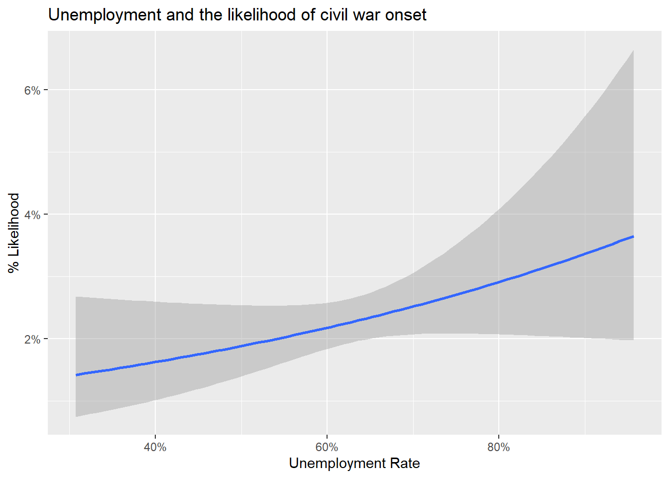

5.3 Bringing in alternative measures of conflict

This ability to merge in new datasets is essential for doing research with any dataset dealing with any topic. For studying conflict in particular, cross-walking and merging datasets can be essential for populating your data with the latest and greatest new variables dealing with conflict itself. A great example is data that comes from the International Conflict Data Project at the University of Alabama. This database is the product of a collaboration between Douglas Gibler and Steven Miller (yes the same Steven Miller responsible for {peacesciencer}). At the moment, the data produced through this collaboration is not directly accessible using {peacesciencer}. This is partly because the data are so new (they came out in summer of 2023). However, with just a few extra steps, the data maintained by the International Conflict Data Project can be easily downloaded and merged with the base datasets you can construct with {peacesciencer}.

Let’s consider, in particular, the Militarized Interstate Events (MIEs) data.¹ The MIE data provide day-level details on militarized events that take place between countries from 1816 to 2014. A militarized interstate event is considered a threat, display, or use of force by one member of the CoW state system toward another. For each MIE, there is a wide variety of information, including details about whether an event is connected to a war (a sustained conflict) and estimates of the minimum and maximum fatalities associated with the event. You can read the MIE code book, which provides all the relevant metadata you would want to know about the dataset (access here: https://internationalconflict.ua.edu/wp-content/uploads/2023/07/MIEcodebook.pdf).

To access the data, you’ll need to download it from the database. You can use this link here: https://www.dropbox.com/s/2aq3xu23a4ril85/events.zip?dl=1. If you click the link, it’ll download a ZIP file to your computer. This file contains five things:

1. A pdf copy of the MIE codebook
2. A pdf of some basic summary statistics based on the data
3. A version of the data as a .csv file
4. … as a .DTA file
5. … as a .RDS file

When you choose where to save this folder in your files, make sure that you save it in the project folder associated with your current R project—specifically in your “Data” folder that I told you to create in the first prerequisite chapter Chapter 2. You’ll then unzip the folder there. It may then be automatically saved inside an “event” folder inside your “Data” folder.

With the data downloaded and unzipped, you can now access the MIE dataset and read it into R. The below code uses the here() function from the {here} package to let me navigate my files in my current R project. I’ve saved the relevant data in my “Data” folder inside a sub-folder called “events.” Of my three choices of data types, I’ve chosen to read in the .csv version of the data.

library(here)
file_location <- here(
  "Data", "events", "mie-1.0.csv"
)
mie_data <- read_csv(file_location)

Rows: 28011 Columns: 18
── Column specification ────────────────────────────────────────────────────────
Delimiter: ","
chr  (1): version
dbl (17): micnum, eventnum, ccode1, ccode2, stmon, stday, styear, endmon, en...

ℹ Use `spec()` to retrieve the full column specification for this data.
ℹ Specify the column types or set `show_col_types = FALSE` to quiet this message.

If we take a quick glimpse at the data object mie_data, we can see that it provides a crazy level of detail for different MIEs over time. In particular, one thing that is clear is that the data is set up at the dyadic level of analysis. This is useful information to know as we think about how we might want to use it in our research.

glimpse(mie_data)

Rows: 28,011
Columns: 18
$ micnum    <dbl> 2, 3, 4, 4, 4, 4, 4, 4, 4, 4, 4, 4, 4, 7, 7, 7, 7, 7, 7, 7, …
$ eventnum  <dbl> 1, 1, 2, 3, 4, 5, 6, 7, 8, 9, 10, 11, 1, 1, 2, 3, 4, 5, 6, 7…
$ ccode1    <dbl> 2, 300, 339, 200, 200, 200, 339, 200, 200, 339, 200, 200, 33…
$ ccode2    <dbl> 200, 345, 200, 339, 339, 339, 200, 339, 339, 200, 339, 339, …
$ stmon     <dbl> 5, 10, 5, 10, 10, 10, 10, 10, 11, 11, 11, 11, 5, 10, 11, 11,…
$ stday     <dbl> -9, 7, 15, 22, 22, 22, 22, 23, 1, 1, 12, 13, 15, 13, 12, 12,…
$ styear    <dbl> 1902, 1913, 1946, 1946, 1946, 1946, 1946, 1946, 1946, 1946, …
$ endmon    <dbl> 5, 10, 5, 10, 10, 10, 10, 10, 11, 11, 11, 11, 5, 10, 11, 11,…
$ endday    <dbl> -9, 7, 15, 22, 22, 22, 22, 23, 1, 1, 12, 13, 15, 13, 12, 15,…
$ endyear   <dbl> 1902, 1913, 1946, 1946, 1946, 1946, 1946, 1946, 1946, 1946, …
$ sidea1    <dbl> 1, 1, 1, 0, 0, 0, 1, 0, 0, 1, 0, 0, 1, 1, 1, 0, 1, 0, 1, 1, …
$ action    <dbl> 7, 1, 16, 7, 7, 7, 16, 7, 7, 16, 7, 7, 16, 7, 7, 8, 17, 16, …
$ hostlev   <dbl> 3, 2, 4, 3, 3, 3, 4, 3, 3, 4, 3, 3, 4, 3, 3, 3, 4, 4, 4, 4, …
$ fatalmin1 <dbl> 0, 0, 0, 0, 0, 0, 0, 0, 0, 0, 0, 0, 0, 0, 0, 0, 1, 0, 0, 0, …
$ fatalmax1 <dbl> 0, 0, 0, 0, 0, 0, 0, 0, 0, 0, 0, 0, 0, 0, 0, 0, 1, 0, 0, 0, …
$ fatalmin2 <dbl> 0, 0, 0, 0, 0, 0, 44, 0, 0, 0, 0, 0, 0, 0, 0, 0, 0, 0, 0, 40…
$ fatalmax2 <dbl> 0, 0, 0, 0, 0, 0, 44, 0, 0, 0, 0, 0, 0, 0, 0, 0, 0, 0, 0, 50…
$ version   <chr> "mie-1.0", "mie-1.0", "mie-1.0", "mie-1.0", "mie-1.0", "mie-…

As we consider how to merge this with a possible universe of observations, we need to be sure to take a couple of things into consideration. Chief among the these is that the MIE dataset itself only has rows for dyad-years for which an MIE took place. It does not have the entire universe of dyad-years in the CoW state system. Second, while we have CoW codes that we can use to match countries in a base dataset constructed with {peacesciencer}, dealing with dates will be an issue. With this second point in mind, it will be helpful to quickly go over what some of the different ID columns signify.

First up is the micnum. This stands for Militarized Interstate Confrontation (MIC) number. Different events can be part of a broader confrontation. This column provides a unique numerical code to distinguish between events that are part of one broader confrontation versus another.

The second ID column is eventnum. This value is not just a numerical code; it has a meaningful interpretation. For a given confrontation, a “1” indicates the first threat, display, or use of force for that particular confrontation. Subsequent numbers indicate the second, third, and fourth events, as applicable.

Next we have the columns ccode1 and ccode2. These of course give the numerical CoW code for side 1 and side 2 of a confrontation.

Following these columns are a set of columns detailing the timing (and conclusion) of a given event based on the month, day, and year.

Using all of these ID columns, we can begin to think about how we’d like to merge this data with a base dataset constructed with {peacesciencer}. We have three options, two of which maximize the amount of detailed information we can make use of in the MIE dataset. The first is to create a dyad-year dataset. {peacesciencer} (wisely) does not allow us to create a day-level version of a dyadic dataset. The size of this data would be unwieldy, requiring a lot of processing power that most people don’t have access to on their personal computer or in a typical online server. If we go this route, the benefit is that we can study MIEs dyadically, taking into consideration both the instigator of an event and the target. The downside is that we’re missing out on day-level variation.

The second base dataset we might consider is at the level of state-days. While {peacesciencer} doesn’t let us study dyads at the day level, we can study countries at the day level. For what it’s worth, when peace science scholars talk about the difference between dyad- and state-level datasets, they sometimes will refer to the latter as a monadic dataset. While a “dyad” means “two,” a “monad” means “one.” A benefit of working with monadic (state-level) data is that we can make use of day-level details about militarized events included in the MIE data. The downside is that we’ll lose information about the other country involved in the event.

Our third option is to construct a monadic dataset at the level of years. This might be a good idea if we don’t care about day-level details about MIEs and we’d just like yearly summaries. An obvious downside with this approach is that we’re missing out on details that the MIE dataset offers us, both in terms of dyadic-level information and in terms of day-level information. However, an upside is that the analysis will be a little simpler to implement.

Whatever we choose to do, we’ll need to take some steps to prep the MIE data before we merge it with a base dataset. There’s no avoiding it. We’ll have to do some data wrangling.

Since we have to make a choice, let’s go with the second option: a monadic dataset at the level of days. The below code uses create_statedays() to create a state-day base dataset using the CoW state system. To make our analysis simple, it then filters the data to dates from the beginning of 2000 to the end of 2014. It then asks R to give us a glimpse of the data.

## create the base data
cow_data <- create_statedays()

## filter to dates from 2000-01-01 onward
cow_data |>
  filter(
    date >= "2000-01-01",
    date <= "2014-12-31"
  ) -> cow_data

## take a look at the data
glimpse(cow_data)

Rows: 1,057,624
Columns: 3
$ ccode    <dbl> 2, 2, 2, 2, 2, 2, 2, 2, 2, 2, 2, 2, 2, 2, 2, 2, 2, 2, 2, 2, 2…
$ statenme <chr> "United States of America", "United States of America", "Unit…
$ date     <date> 2000-01-01, 2000-01-02, 2000-01-03, 2000-01-04, 2000-01-05, …

You’ll notice from the output with glimpse() that in this is a large dataset. It has almost 1.7 million rows. Just imagine how large this would be if it were a dyadic dataset! You’ll also notice that our cow_data object has three columns: ccode, statenme, and date. The first two are the same as what we’d get with a state-year dataset, but the date column is new. R has a number of different data classifications that determine how it handles that data. In this case, the values in the date column are classified as, well, dates. Just to confirm, we can use the class() function to ask R to tell us the class of the date column. Sure enough, the column is of class “Date.”

class(cow_data$date)

[1] "Date"

Now that we have our base data, which is a monadic dataset, we need to wrangle the MIE data into the right size to match the other’s monadic structure. We’ll also need to cross-walk the dates to align with those in the date column in the base dataset. The below code performs the necessary operations on the mie_data object to make this happen. I’ve provided annotations in my code to specify what I’m doing and why. The end product is a data object called md_mie_data that is a monadic-day level dataset.

## start with the mie data and pipe into mutate
mie_data |>
  ## create a new date column
  mutate(
    ## -9 in stday means the day is missing
    ## when this is the case treat it like the 
    ## 1st day of the month
    stday = ifelse(stday == -9, 1, stday),
    ## paste the year, month, and day together
    ## in year-month-day format then tell
    ## R that the output is a set of dates
    date = paste0(
      styear, "-",
      str_pad(stmon, width = 2, pad = "0"), "-",
      str_pad(stday, width = 2, pad = "0")
    ) |> as.Date()
  ) |>
  ## first aggregate the data to the level of MICs,
  ## ccode1, and dates
  group_by(ccode1, date, micnum) |>
  reframe(
    ## for each MIC, get the number of events,
    ## whether a country initiated
    ## the hostility level (1-5 scale)
    ## sum of min. & max. fatality estimates 
    n_mie = length(unique(eventnum)),
    n_initiated = unique(sidea1),
    hostlev = unique(hostlev),
    fatalmin = sum(fatalmin1),
    fatalmax = sum(fatalmax1)
  ) |>
  ## now aggregate to the level of state-days
  group_by(ccode1, date) |>
  reframe(
    ## for each state-day get a count of:
    ## - no. of MICs
    ## - no. of MIEs
    ## - no. of MICs initiated
    ## - max hostility level on a given day
    ## - no. of min. estimated fatalities
    ## - no. of max. estimated fatalities
    n_mic = length(unique(micnum)),
    n_mie = sum(n_mie),
    n_initiated = sum(n_initiated),
    hostlev = max(hostlev),
    fatalmin = sum(fatalmin),
    fatalmax = sum(fatalmax)
  ) |>
  ## one last thing. change the name of
  ## the ccode1 column to ccode
  rename(
    ccode = ccode1
  ) -> md_mie_data

## make sure that there are no duplicate rows
md_mie_data |>
  nrow() -> no_of_rows
md_mie_data |>
  select(ccode, date) |>
  nrow() -> no_we_want
no_of_rows == no_we_want ## We're good!

[1] TRUE

With our cleaned up version of the MIE dataset, we can now merge it with the {peacesciencer} base dataset we created.

cow_data |>
  left_join(
    md_mie_data,
    by = c("ccode", "date")
  ) -> cow_data

We’re now good to go. Let’s do a quick analysis summarizing some daily trends in international conflict. First, what is the daily number of countries involved in at least one militarized interstate event from the beginning of 2000 to the end of 2014?

cow_data |>
  group_by(date) |>
  reframe(
    n_mie = sum(n_mie >= 1, na.rm = T)
  ) |>
  ggplot() +
  aes(
    x = date,
    y = n_mie
  ) +
  geom_line() +
  labs(
    x = "Date",
    y = NULL,
    title = "Daily no. countries involved in MIEs, 2000-2014"
  )

We can also summarize the daily range of estimated fatalities from all MIEs during the 2000 to 2014 period. For example, we can check out the maximum estimated daily fatality count from all MIEs between 2000 and 2014:

cow_data |>
  group_by(date) |>
  reframe(
    fatalmax = sum(fatalmax, na.rm = T)
  ) |>
  filter(
    fatalmax > 0
  ) |>
  ggplot() +
  aes(x = date, y = fatalmax) +
  geom_point() +
  geom_smooth() +
  scale_y_log10(
    labels = scales::comma
  ) +
  labs(
    x = "Date",
    y = NULL,
    title = "Daily no. of max. fatalities from all MIEs"
  )

`geom_smooth()` using method = 'loess' and formula = 'y ~ x'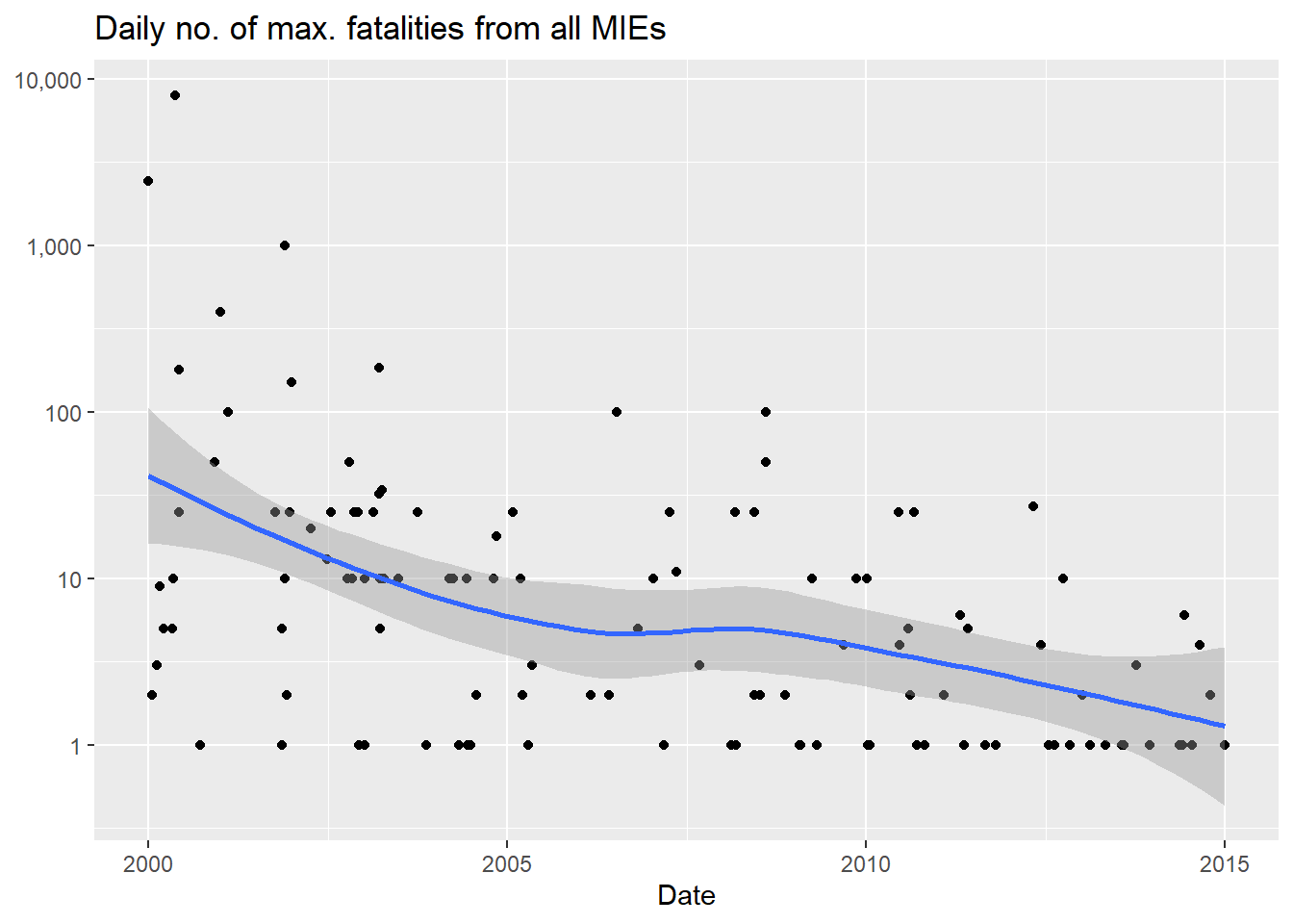

Day-level detail like this can be really useful for a number of research designs. For example, you might be interested in conducting a regression discontinuity or difference-in-differences research design where you cross-reference day-level events with MIE data to infer causal effects. As a really simple example of the former, say we wanted to know whether Barack Obama’s ascension to the US Presidency led to a significant change in the number of new MIEs the US was involved in. The below code filters the data down to the US. It then sets up what we need for a very simple regression discontinuity design. It creates a “treatment” variable that takes the value of 1 for all days from Obama’s inauguration (Jan. 20, 2009) onward. It then models the pre- and post-Obama trend in MIEs for the US using a Poisson model with a non-linear time trend. Just as the logit model we discussed in the previous chapter is an extension of the standard linear model for binary data, the Poisson model is an extension used for count data. As you can see, there’s not really a statistically significant change in the number of MIEs the US was involved in post-Obama. If anything, the number of MIEs the US was involved in was really just a continuation of a trend that started under the Bush Administration (as an exercise, you might try alternative models to see how the results change).

library(geomtextpath)
cow_data |>
  filter(
    ccode == 2
  ) |>
  mutate(
    treatment = ifelse(
      date >= "2009-01-20",
      1, 0
    ),
    n_mie = replace_na(n_mie, 0)
  ) |>
  ggplot() +
  aes(
    x = date,
    y = n_mie
  ) +
  stat_smooth(
    method = "gam",
    method.args = list(family = quasipoisson),
    aes(group = treatment)
  ) +
  geom_textvline(
    aes(xintercept = min(date[treatment==1])),
    label = "Obama Takes Office",
    hjust = 0.8
  ) +
  labs(
    x = "Date",
    y = "No. MIEs (Poisson Model)",
    title = "US involvement in MIEs before and after\nObama's inauguration in 2009"
  ) 

`geom_smooth()` using formula = 'y ~ s(x, bs = "cs")'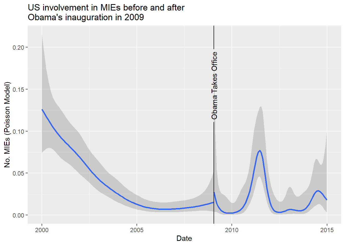

5.4 Wrapping up

Given the sheer number of datasets you might want to incorporate in your analysis, it is impossible for me to write a truly comprehensive guide on cross-walking and merging external datasets with the core functions of {peacesciencer}. However, knowing how to use the countrycode() function from the {countrycode} package will equip you to work with most of the datasets you might run into.

Also, many external datasets may be in the wrong shape for your analysis. Rarely will you be able to avoid doing any data wrangling prior to cross-walking and merging datasets. Starting with {peacesciencer} to construct your base data will make this process much easier. One of the hardest aspects of wrangling data isn’t the technical details (however, those can be tricky); it’s the conceptual details. These include what you’d like your data to look like in terms of the unit of analysis and unit of time. By starting out with a base dataset constructed using tools from {peacesciencer}, you can work out the conceptual details first. That way, whatever new data you’d like to bring in to your analysis, you know what you want the final product of your data wrangling to look like.

In the next chapter, we’ll practice some more data wrangling and explore many popular correlates of conflict.

Arel-Bundock, Vincent, Nils Enevoldsen, and CJ Yetman. 2018. “Countrycode: An r Package to Convert Country Names and Country Codes.” Journal of Open Source Software 3 (28): 848.

Gibler, Douglas M, and Steven V Miller. 2023. “The Militarized Interstate Events (MIE) Dataset, 1816–2014.” Conflict Management and Peace Science, 07388942231182674.

---

1. Read more about it in Gibler and Miller (2023).