The previous part of these notes was dedicated to studying five reasons for war discussed by Blattman (2023). In this part of the notes, we’ll transition to discussing four pathways to peace that he discusses as well. The first of these pathways is interdependence. Interdependence helps to promote peace by increasing the costs of war. The standard bargaining model of war assumes that the sides of a dispute only have private benefits from getting a larger share of some prize and private costs from going to war to fight for that prize. However, these benefits and costs are not always private. Sometimes what is good for one group or country is also good for another. Similarly, what is bad for one group or country is also bad for another.
Interdependence can take on many forms. The three discussed by Blattman (2023) are:
Economic: Factors like trade, investment, and business relationships are mutually beneficial for those involved (generally). War is usually bad for business, so when groups are economically intertwined the choice to go to war can be much higher than when groups share few economic ties.
Social: Social contact between groups can improve their relationships with each other, causing them to see members of another group as friends rather than foes. The denser the social bonds between groups, the more a war would be perceived has costly and unthinkable.
Cultural: Having a shared culture or identity can expand the circle of your in-group to include individuals from a wide range of racial, ethnic, and religious backgrounds. These cultural linkages can make war prohibitively costly.
Each of the above three need not be mutually exclusive. They can work in concert, complementing each other and, thereby, can make peace all the more attractive. The primary reason these factors contribute to peace is their effect on the cost of war. By making war more costly for both sides of a dispute, this expands the bargaining range. This is no guarantee that sides will always be able to find peaceful compromises, but it does increase the odds.
How can we go about testing the role of interdependence as a driver of peace with data? A good place to start is international trade. The level of trade between countries can be a good indicator of their economic interdependence. By extension, it might be able to explain variation in international conflict. In this chapter, we’ll walk through an example with {peacesciencer} examining the role of trade as an explanatory variable for conflict.
13.1 Hypothesis
Gartzke (2007) and many other conflict scholars refer to the idea that economic ties reduce the likelihood of conflict as the capitalist peace. The capitalist peace makes a very simple prediction: more trade leads to more peace. This idea is not new. Philosophers such as Montesquieu, Paine, and Mill believed in the power of commerce to lead to peace because of the increased material benefits that all enjoy through peaceful exchange. If this is true, then we should expect the following hypothesis to be supported:
Hypothesis 1: Greater trade between dyads or pairs of countries will decrease the likelihood of militarized disputes between them.
However, before we go to the analysis, we should think a little more carefully about this hypothesis and whether trade levels are fully capturing the concept of economic interdependence. First, it is possible that trade is correlated with the frequency of country interactions in general, and countries that interact more often may be more apt to go to war simply because of this regular interaction. This might lead us to observe a positive relationship between trade and conflict rather than a negative one.
Second, while trade surely matters for peace, different pairs of countries can have different levels of trade dependence which will influence the relative cost of war for one side versus the other. For example, if country A has a large economy but B has a small economy, a certain level of trade may be relatively more important for B than for A. The idea is that lost revenue from trade will have a larger impact on B’s economy than A’s. If one side is especially dependent on trade relative to the other, this might influence prospects for peace. In particular, it could be that:
Hypothesis 2: The more one side is dependent on trade relative to the other, the lower the likelihood that it initiates a conflict with the other side.
This hypothesis, if supported by the data, may indicate that interdependence has a dark side. The more one side depends on another, the more likely it may be to accept less generous terms in a bargain. In short, dependence might spur peace in addition to, or instead of, interdependence. Conversely, the less one side is dependent on trade with the other, the more likely it may be to initiate a conflict.
13.2 Data
To test these hypotheses, we’ll put together a directed dyad-year dataset. The reason for using a directed dyadic dataset is that hypothesis 2 in particular requires us to consider the identity of the country initiating a dispute. The below code puts together the data. It begins with a base dyadic year dataset and then populates it with conflict data, data about peace spells, data about dyadic distances, and data about country GDP. We need the latter to help us construct a measure of trade dependence. We need the former as a control variable. More proximate countries may have a higher likelihood of going to war and of engaging in trade, so we need to account for this in our statistical model. There is also a line of code that uses the readRDS() function to read in directed dyad trade data from Steve Millers website. There is an add_cow_trade() function included with {peacesciencer} that would normally be used to populate this data with dyadic trade flows. However, depending on the system an R user is working with (an online R server versus RStudio for desktop) there are some permission issues that rear their ugly head in accessing this data. So the below code provides a replicable work around that should work regardless of the permissions in your particular environment:
## packages + setuplibrary(tidyverse)library(peacesciencer)library(sandwich)library(lmtest)library(coolorrr)set_theme()set_palette()## create the datacreate_dyadyears(directed = T,subset_years =1870:2010) |>add_gml_mids() |>add_spells() |>add_sdp_gdp() |>add_minimum_distance() |>filter_prd() -> Data
Joining with `by = join_by(ccode1, ccode2, year)`
Joining with `by = join_by(ccode1, ccode2, year)`
add_gml_mids() IMPORTANT MESSAGE: By default, this function whittles
dispute-year data into dyad-year data by first selecting on unique onsets.
Thereafter, where duplicates remain, it whittles dispute-year data into
dyad-year data in the following order: 1) retaining highest `fatality`, 2)
retaining highest `hostlev`, 3) retaining highest estimated `mindur`, 4)
retaining highest estimated `maxdur`, 5) retaining reciprocated over
non-reciprocated observations, 6) retaining the observation with the lowest
start month, and, where duplicates still remained (and they don't), 7) forcibly
dropping all duplicates for observations that are otherwise very similar. See:
http://svmiller.com/peacesciencer/articles/coerce-dispute-year-dyad-year.html
Warning in xtfrm.data.frame(x): cannot xtfrm data frames
Joining with `by = join_by(orig_order)`
Joining with `by = join_by(ccode1, ccode2, year)`
Joining with `by = join_by(ccode1, ccode2, year)`
## read in trade datareadRDS(url("http://svmiller.com/R/peacesciencer/cow_trade_ddy.rds")) -> trade_dt## merge the trade data with the main dataData |>left_join( trade_dt ) -> Data
Joining with `by = join_by(ccode1, ccode2, year)`
With the dataset constructed, we now need to make some updates to the variables for trade flows tend to have a skewed distribution, meaning some outliers might overly influence the results. The code below creates a function called rescale() that will transform the data by first, converting it to ranks rather than the raw numerical values, rescaling these from 1 to 10, and then taking the natural log. I then use this function to help in the construction of two trade variables that we will use in the analysis:
lrank_trade: the logged rescaled rank transformation of total bilateral trade between country 1 and country 2
lrat_trade_dep1: the logged rescaled rank transformation of side 1’s trade dependence relative to side 2’s
## create measures for analysis# rescaling functionrescale <-function(x) { x <-rank(x) x <- x -min(x, na.rm = T) x <- x / (max(x, na.rm = T)) x <-log(x *9+1) x}# make changesData |>mutate(# treat NA = 0 for tradeacross(flow1:flow2, ~replace_na(.x, 0)),# make dyad indicatordyad =paste(ccode1, ccode2, sep ="-"),# measure of total tradetotal_trade = flow1 + flow2,# the log-rank of total tradelrank_trade =rescale(total_trade),# trade dependence of side 1 and 2trade_dep1 = (1000000* total_trade) /exp(wbgdp2011est1),trade_dep2 = (1000000* total_trade) /exp(wbgdp2011est2),# log ratio of side 1 trade dependencelrat_trade_dep1 =rescale(trade_dep1) -rescale(trade_dep2),# log-rank of dyadic distancelrank_dist =rescale(mindist) ) -> Data
13.3 Analysis
To test hypothesis 1 and 2 we’ll estimate a logit model where the likelihood that side 1 initiates a MID is the outcome and the trade variables we created above are the main predictors of interest. We’ll also control for the logged rescaled bilateral distance between country 1 and country 2 and a cubic peace spell trend. This is done in the below code and the model fit is saved as an object called model_fit.
Using a combination of coeftest() and vcovCL() we can check out the results using robust-clustered standard errors for the model estimates. This is done in the following code. What do you notice about the results? Do we have support for the hypotheses? The answer is a big fat NO. We have support for hypothesis 2 (the more side 1 is trade dependent on side 2, the less likely it is to initiate a MID with side 2), but the data supports the opposite conclusion of what hypothesis 1 predicts (rather than more trade leading to more peace, it makes side 1 more likely to start a MID with side 2).
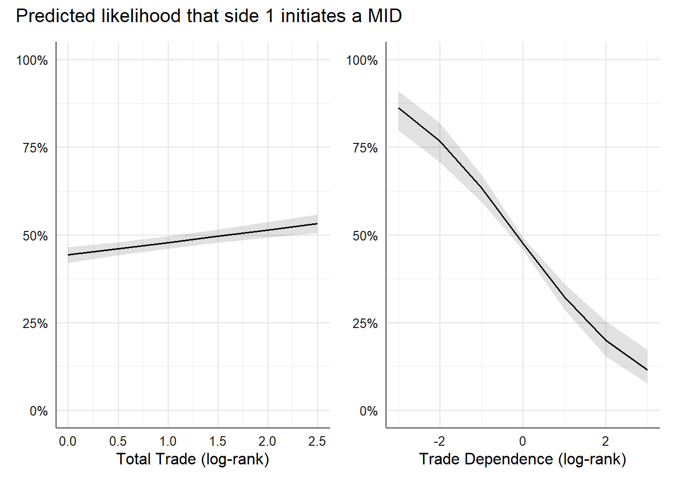
As usual, since we’re dealing with a generalized linear model, it’s often much easier to get a sense for what the model is telling us by visualizing the relationships implied by the model. The below code plots the predicted % likelihood of that side 1 initiates a MID with side 2 based on their level of bilateral trade and side 1’s trade dependence on side 2. These values show that the negative impact of trade dependence is quite substantial whereas the impact of total trade is modest.
Scale for y is already present.
Adding another scale for y, which will replace the existing scale.
Scale for y is already present.
Adding another scale for y, which will replace the existing scale.
What should we make of these results? On the one hand, it could be that the more countries trade the more they have to fight about. It could also be a fluke due to our failure to account for factors that trade is correlated with that might also explain war. For example, more trade may equal more power. Whatever the explanation, the plain fact is that, over time, countries that trade more with each other also seem to be more conflictual.
At the same time, much of the conflict that is explained by trade seems to be a result of asymmetries in trade dependence. While trade dependent countries are unlikely to initiate MIDs with major trade partners, the reverse is true for countries that are in a position of power relative to a trade partner. This suggests a possible dark side to trade.
13.4 Conclusion
Interdependence is a plausible means to peace, as evidenced by numerous examples discussed by Blattman (2023). However, when we examine a form of interdependence (economic interdependence through trade) at the international level, evidence of its peace-building properties doesn’t materialize. If anything, stronger economic ties at the international level seem to make countries more conflict-prone rather than less. Further, while it is true that trade dependence makes countries less likely to start fights, trade dominance makes countries more likely to do so.
This analysis, importantly, is not a rigorous refutation of the claims Blattman (2023) makes. Remember, the goal with these exercises is to use the frameworks laid out by Blattman (2023) to motivate data-based examples (and that is all). Moreover, there are many forms of interdependence beyond trade, even within the economic sphere that we haven’t considered, such as foreign investment. We also haven’t examined social or cultural interdependence, which might also help explain patterns in international conflict. Looking at such factors might make for useful and interesting extensions on the analysis presented here. For example, it might be instructive to look at patterns in international migration as a proxy for social ties, or common language and religion as proxies for culture. Such data are not available with {peacesciencer} but there are many such sources of data available elsewhere.
Blattman, Christopher. 2023. Why We Fight: The Roots of War and the Paths to Peace. Penguin.
Gartzke, Erik. 2007. “The Capitalist Peace.”American Journal of Political Science 51 (1): 166–91.