Up to now, we’ve studied four reasons for war—unchecked interests, intangible incentives, uncertainty, and commitment problems. In this chapter, we’ll consider the fifth and final reason for war that Blattman (2023) discusses in his book: misperceptions.
Misperceptions deal with different kinds of biases that influence (and sometimes hijack) our rational thinking. These biases are a product of mental shortcuts our brains take in drawing conclusions and making sense of events and information. The world is a complicated place, and to spend time in deep contemplation about every facet of the world is practically impossible. In fact, it’s advantageous for our survival that we have the ability to draw quick conclusions and act with speed when confronted with emergencies or fast developing crises.
This kind of thinking is what the famed psychologist Daniel Kahneman calls “fast thinking.” However, while fast thinking confers an evolutionary advantage for our species, when we’re engaged in fast thinking we often miss important bits of information. This creates space for errors in judgment or action. Furthermore, these errors aren’t just random. One of the most significant findings to come out of the field of behavioral science is that these errors are systematic and predictable. That is, we humans consistently make the same mistakes when confronted with situations that trigger fast thinking. We call these systematic mistakes cognitive biases.
As Blattman (2023) discusses, the misperceptions or cognitive biases that we fall prey to under certain conditions can lead to hasty actions or missteps that ultimately lead groups or countries down a path toward war. While Blattman provides a rich set of examples that demonstrate how cognitive biases warp our thinking, the goal in this chapter is to consider how we might be able to test the role of such biases in leading to war more systematically, using data. To do this, we need to first consider what factors in the world we can measure that might tell us something about variation in misperceptions. Misperceptions are impossible to measure directly. To do so, we would need to see inside the minds of decision-makers at critical junctures in their interactions with adversaries. Instead, we need to think creatively in order to identify different conditions under which space for misperceptions to influence decisions to go to war will likely be present. This chapter walks through an example using {peacesciencer} where we can try to triangulate instances where misperceptions are likely to influence decision-makers.
12.1 Hypothesis
There are three kinds of misperceptions that Blattman (2023) argues are the most problematic for preserving peace:
Overconfidence
Misprojection
Misattribution
Overconfidence can lead to war if leaders underestimate uncertainty about their power versus their adversary, or if leaders overestimate their own ability. Misprojection can lead to war if leaders mistakenly project their own motives on to other actors. Misattribution can lead to war if leaders assume the worst about the other side.
For the below analysis, we’ll focus on the first of these misperceptions (overconfidence). Overconfidence in particular has an empirical implication that Blattman (2023) already hints at in his book:
Hypothesis: Leaders with military training but no combat experience are more likely to start militarized disputes than leaders with military training and prior combat experience.
The reason behind this expectation is simple. Leaders with military training and no combat experience will be overconfident about going to war. These leaders may know a lot about the theory of going to war, but they lack real-world experience with the trials and tribulations of combat. As a result, they are likely to overestimate their country’s ability to achieve swift victory while they underestimate the potential costs of fighting. Let’s see if this line of reasoning holds up in the data.
12.2 Data
To test the role of overconfidence in leading to war, we’ll construct a leader-year dataset and populate it with data about conflict initiation and leader attributes. The below code opens the {tidyverse} and {peacesciencer} packages and then creates a base dataset at the leader-year level of observation. It then pipes this base data into functions that add information about militarized interstate disputes (MIDs), peace spells, and leader attributes from the LEAD project dataset.
## open {tidyverse} and {peacesciencer}library(tidyverse)library(peacesciencer)## create the datacreate_leaderyears(standardize ="cow",subset_years =1875:2010) |>add_gml_mids() |>add_spells() |>add_lead() -> Data
Joining with `by = join_by(gwcode, year)`
Joining with `by = join_by(ccode, date)`
Joining with `by = join_by(gwcode, year)`
Joining with `by = join_by(ccode, date)`
Joining with `by = join_by(ccode, date)`
Joining with `by = join_by(obsid, year)`
Warning in xtfrm.data.frame(x): cannot xtfrm data frames
Joining with `by = join_by(orig_order)`
Warning in xtfrm.data.frame(x): cannot xtfrm data frames
Joining with `by = join_by(orig_order)`
Joining with `by = join_by(obsid)`
This dataset that we’ve constructed has a number of variables about leaders. We’ll focus on two to test the hypothesis proposed in the previous section:
milservice: 1 if the leader has previous military service and 0 otherwise
combat: 1 if the leader has previous combat experience and 0 otherwise
There are many other details about leaders in the data as well, such as education and mental health. If you like, these also worth exploring on your own, because they may also correspond with different kinds of misperceptions that leaders could be susceptible to.
12.3 Analysis
With our data compiled, let’s see if our hypothesis that leaders with military training but no combat experience are prone to starting more MIDs than other leaders. To do this, we’ll estimate a logistic regression model with an interaction term for military service and combat experience. Formally, our regression model is specified as follows:
The value \(p_{it}\) represents the probability that a leader \(i\) starts a MID with another country in year \(t\), and the expression \(f(s_{it})\) represents a cubic peace spells trend. The variables of interest include the indicator for prior military service and the indicator for prior combat experience. You may notice that these variables enter the regression equation in an interesting way. First, observe that military service is multiplied by 1 minus combat experience and that combat experience then enters the model as its own separate term. Using this specification, the value of \(\beta_1\) will tell us how the logged-odds of MID initiation changes for leaders with prior military service but no combat experience while \(\beta_2\) will tell us how the logged-odds of MID initiation changes for leaders with military service and prior combat experience. The reason we can enter these variables into the model in this way is that there are no cases in the data where a leader has prior combat experience but no prior military service. To confirm, we can use the table() function to quickly produce a cross-tabulation of instances for different combinations of military service and combat experience. As you can see below, the category for combat experience but no military service has zero observations in the data.
table(Data$milservice, Data$combat)
       0    1
  0 8974    0
  1 1426 3472
To estimate the model, we’ll use glm(). The code below estimates the model and saves the output as a object called logit_fit. To make estimating the model specified above easier, add a column to the data along the way called service_factor that represents the three possible categories a leader could fall into with respect to their prior military service and combat experience. I then use this variable as the main predictor in the regression model.
library(socsci)
Loading required package: rlang
Warning: package 'rlang' was built under R version 4.2.3
Attaching package: 'rlang'
The following objects are masked from 'package:purrr':

    %@%, flatten, flatten_chr, flatten_dbl, flatten_int, flatten_lgl,
    flatten_raw, invoke, splice
Loading required package: scales
Warning: package 'scales' was built under R version 4.2.3
Attaching package: 'scales'
The following object is masked from 'package:purrr':

    discard
The following object is masked from 'package:readr':

    col_factor
Loading required package: broom
Warning: package 'broom' was built under R version 4.2.3
Loading required package: glue
Data |>mutate(service_factor =frcode( milservice ==0~"No Military Service", milservice * (1- combat) ==1~"Service with No Combat", combat ==1~"Service with Combat" ) ) -> Dataglm( gmlmidonset_init ~ service_factor +poly(gmlmidinitspell, 3),data = Data,family = binomial) -> logit_fit
In previous code, we’ve used {mfx} to estimate logit models since it lets us compute robust-clustered standard errors. However, we have other options as well by using tools from {sandwich} and {lmtest}. The below code shows how to use these tools and reports the model results. Consistent with the hypothesis, the estimate for leaders with military experience but no combat experience is greater than the estimate for leaders with military experience and combat experience. However, both are statistically significant and positive, suggesting that any military service makes leaders more apt to go to war. In other words, while prior combat experience tempers leader willingness to start fights, it doesn’t totally eliminate it.
z test of coefficients:

                                       Estimate Std. Error  z value  Pr(>|z|)
(Intercept)                           -2.137697   0.055909 -38.2356 < 2.2e-16
service_factorService with No Combat   0.523673   0.134235   3.9012 9.573e-05
service_factorService with Combat      0.428877   0.094874   4.5205 6.169e-06
poly(gmlmidinitspell, 3)1            -61.996565   9.262236  -6.6935 2.179e-11
poly(gmlmidinitspell, 3)2             16.489789  18.338454   0.8992   0.36855
poly(gmlmidinitspell, 3)3            -26.643440  15.786264  -1.6878   0.09146

(Intercept)                          ***
service_factorService with No Combat ***
service_factorService with Combat    ***
poly(gmlmidinitspell, 3)1            ***
poly(gmlmidinitspell, 3)2
poly(gmlmidinitspell, 3)3            .
---
Signif. codes:  0 '***' 0.001 '**' 0.01 '*' 0.05 '.' 0.1 ' ' 1
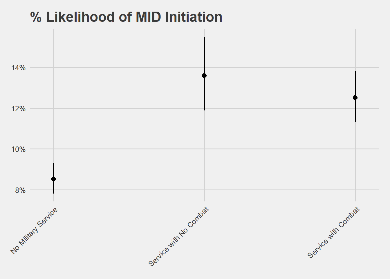
We can use plot_model() from {sjPlot} to show what the practical implications of these model estimates are for the expected likelihood that a leader starts MIDs. The below code produces predictions from the model of the effect of military experience depending on whether a leader also has prior combat experience. Note that it also lets us specify that we want cluster-robust standard errors using the same vcovCL() function we used to look at the model output above. In both cases, you can see that military service increases the likelihood that a leader initiates a MID in a given year. However, you can also see that prior military service has a somewhat attenuated relationship with MID initiation if a leader also has combat experience. Importantly, the evidence supports the idea that prior military training without actual combat experience makes leaders more prone to initiating fights with other countries relative to having prior combat experience. However, the difference combat experience makes is not profound.
The above analysis provides some support for the idea that misperception can play a role in leading to war. Of course, there are many other ways that we could capture misperception with data, and these other ways might reveal a conflicting picture. Nonetheless, it is the case that misperceptions, and overconfidence in particular, can explain why some wars start.
At this point, it seems clear that many factors can lead to war, but is there anything that can be done to make peace more likely? The next section of this book will turn to what Blattman (2023) has to say about paths to peace. He highlights four in particular, each of which we’ll consider using data.
Blattman, Christopher. 2023. Why We Fight: The Roots of War and the Paths to Peace. Penguin.