6 Making the Most of {peacesciencer} and Data Analysis Tools in R
In this final chapter dealing with what you need to know to get started with research using {peacesciencer}, I’d like to give you some tips on how to make the most of what the package has to offer. In the coming chapters, we’ll walk through a number of applied examples focusing on substantive questions about the causes of war and paths to peace as outlined by Blattman (2023) in Why We Fight. While I hope you find these substantive examples useful, I want to make sure we start off on the right foot. While I can’t tell you everything there is to know about each and every variable you can access using {peacesciencer}, I can give you some tips for exploring your options with the package—for example, with accessing help files for different functions and other data documentation.
I also want to briefly cover common statistical techniques used in peace science research. The word briefly should be emphasized because my goal is not to offer a comprehensive tutorial on statistical analysis. There are many great resources on this topic already (many of which are free). If you’d like to learn more, I’ve provided some references at the conclusion of this chapter. Consider my summary more of a crash-course in regression analysis with a narrow focus on conflict research. I won’t be able to cover everything you might want to know, but I want to cover enough so that you can get started.1
6.1 Making the Most of {peacesciencer}
Every function in R has a help file that tells you anything you might want to know about a function, how to use it, and what to make of its output. To access a particular function’s help file, all you need to do is write and run ?function_name in the R console. When you do, a help file will open under the “Help” tab (usually in the bottom right pane in RStudio).
This also applies for all functions and some specific datasets in {peacesciencer}. Want to learn more about what the function add_gml_mids() does? Just ask for the help file by writing and running ?add_gml_mids() in the console.
Of course, a prerequisite for asking R for a help file for a function is that you know a particular function exists. Thankfully, {peacesciencer}, in addition to having thorough documentation accessible directly within the RStudio IDE, has an extensive webpage that covers all kinds of details about how certain functions work under the hood and how you can use different “hacks” to cajole the data into formats not explicitly supported with the package’s core functions. More to the point, it has a page that provides a quick reference for every function and dataset that you have access to with the package, which you can access here: https://svmiller.com/peacesciencer/reference/index.html. For each function and dataset, there’s a quick summary as well as a link that will take you to a help file that provides more detailed information.
On the subject of detailed information, I personally find the documentation for the data files helpful in understanding the strengths and weaknesses of different variables. Some datasets, like Leader Willingness to Use Force (lwuf), have several alternative measures of a single concept, and it often isn’t clear which among these alternatives is the best to use. Mercifully, the data documentation provides some context for alternative measures and offers guidance about which you might want to consider using. With respect to leader willingness to use force, there are four measures, and if you look at the data itself, these measures have uninformative names (theta1_mean, theta2_mean, theta3_mean, and theta4_mean). No big deal! The help file offers clarity:
The letter published by the authors [Carter and Smith, who created the data] contains more information as to what these thetas refer. The “M1” theta is a variation of the standard Rasch model from the boilerplate information in the LEAD data. The authors consider this to be “theoretically relevant” or “risk-related” as these all refer to conflict or risk-taking. The “M2” theta expands on “M1” by including political orientation and psychological characteristics. “M3” and “M4” expand on “M1” and “M2” by considering all 36 variables in the LEAD data.
The authors construct and include all these measures, though their analyses suggest “M2” is the best-performing measure.
The documentation offers an elevator pitch about the different measures in the data and provides some guidance on which one you might want to start with. Furthermore, since details about the original source data are provided, you know where you can go to get more details about how the data were constructed.
It bears noting that nowhere in the help files is there a set of instructions for what kind of research questions you should ask or analyses you should do. It is up to you to come up with questions and to seek answers to those questions using your best judgment. I will tell you, though, that one of the best ways to come up with a research question and a research design for answering it is to read through some of the cited works associated with different datasets accessible with the {peacesciencer} package. At the bottom of each help file there are references associated with each dataset. In most cases, the studies cited in the references offer one or more applied examples of ways to use a particular dataset. If a reference is for a relatively recent study, you may even be able to get a sense for what lingering questions or gaps in knowledge exist on a particular problem. If it interests you, use this as your cue to see if you can fill that gap.
6.2 Data analysis choices
Once you have your data (and ideally a research question), the next step is to come up with a research design. A research design is just a plan for how you’ll analyze your data to test a hypothesis (or hypotheses) or, more informally, explore it to generate new hypotheses or new insights.
When it comes to studying conflict with data, the scope of what you can do in terms of research design is somewhat limited, which can be either a source of relief or frustration. We can’t study war in a laboratory under controlled conditions. Nor can we conduct randomized trials of different policy interventions to see how they impact the probability of new wars breaking out. The best we can do is collect good quality observational data and draw inferences from a set of methods that, however sophisticated, boil down to correlational analysis.
Don’t let the limited scope of research designs that are applicable for conflict research mislead you into believing you’re excused from having to think carefully about your analysis choices. The are still several important decisions you need to make:
What is my research question?
Do I have the data that I need to answer this question, and is it of good quality?
What is the scope of my study in terms of the unit of analysis and the time-frame considered?
What variables or factors do I need to adjust for so that I’m making the most appropriate comparisons for answering my research question?
What statistical model should I use to efficiently capture variation in my outcome of interest while minimizing bias?
I could list a few more questions, but these five—(1) research question, (2) data, (3) scope, (4) adjustment strategy, and (5) statistical model—are a good place to start. Up to now, we’ve addressed the first three in some form or fashion. Thought a tutorial on (1) is outside the scope of what I intend to do with this guide book—it’s really up to you to discover what questions or problems in the world most interest you—in the previous chapters and those to come, I hope you find some inspiration. With respect to (2), no data are perfect, but I hope you realize {peacesciencer} offers access to a number of data sources that are of good quality (certainly some of the best that political science has to offer). For (3), the {peacesciencer} package’s six core functions for building a base dataset will take you a long way. While they cannot tell you what your universe of cases should look like, they’ll let you reliably create this universe of cases in a transparent and reliable way.
This leaves questions (4) and (5). The way to answer (4) is to consider how best to compare apples to apples. If you’re interested in whether leader willingness to use force has any bearing on whether a country is more likely to start fights with other countries, you might want to consider what other factors are correlated with willingness to use force such as democracy, economic development, alliances with other countries, or participation in international organizations. These factors might also influence how likely a country is to start a fight. Therefore, assessing the relationship between leader willingness to use force and conflict initiation without adjusting for these other factors might give you misleading results.
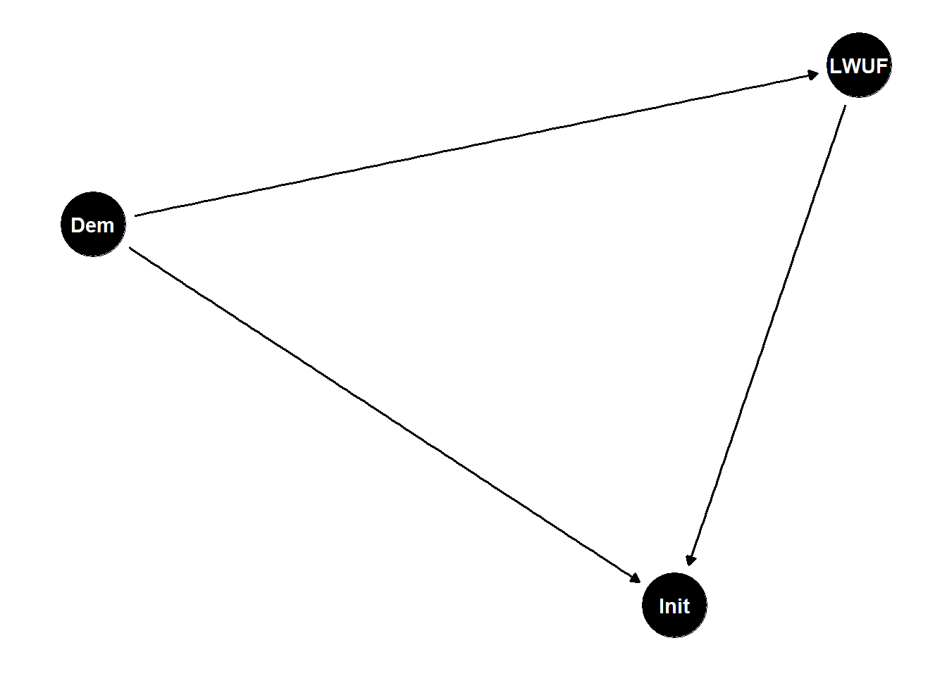
A good approach going into an analysis is to draw what’s called a Directed Acyclic Graph (DAG), which is a fancy name for what is essentially a diagram of our assumptions about the relationships between different factors in the world. The below figure offers a really simple example dealing with leader willingness to use force, democratic governance, and conflict initiation. In it, we assume that while leader willingness to use force influences conflict initiation (based on the direction of the arrows), democracy both influences leader willingness to use force and conflict initiation. The term we would use to describe democracy is confounder, because by failing to account for it in our analysis it would confound or obscure the true impact of leader willingness to use force on the likelihood of conflict initiation. Therefore, given our assumptions about how these three factors are related to each other, we would be wise to adjust for democracy in our analysis.
Keeping with this example, knowing what we need to control for to test whether leader willingness to use force plays a role in international conflict, we now need to choose a statistical model. There are many choices out there. For now, I would like to draw your attention to two commonly used options in peace science research: the logit model and the Poisson model.
In political science, the workhorse method for data analysis is the multiple regression model. Regression analysis has diverse purposes. It can be useful for making forecasts, it can be used to draw descriptive inferences about correlations, and it can be used to make causal inferences.
A discussion of regression usually starts with the classic linear regression model, which is specified with an equation that looks something like this:
\[ y_i = \beta_0 + \beta_1 x_i + \epsilon_i \]
If you’re paying attention, you’ll notice that this has a passing resemblance to the classic linear equation you would have learned in linear algebra:
\[ y = mx + b \]
The basic idea is that we have some outcome variable, \(y\), that is linearly explained by variation in an explanatory variable, \(x\), plus some random or unexplained noise, \(\epsilon\). This simple model can be generalized to accommodate many different variables beyond \(x\). This more general model is called a multiple regression model (not to be confused with a multivariate regression model, which is a model with multiple outcomes), and it looks something like this:
\[ y_i = \beta_0 + \beta_1 x_{i1} + ... + \beta_k x_{ik} + \epsilon_i = \beta_0 + x_i^\top \beta + \epsilon_i \]
Using a method called ordinary least squares (OLS), you can calculate the \(\beta\)s of the linear regression model. You can also calculate them using a variety of other methods, but OLS is the most common.
You can estimate a linear model using OLS with the lm() function in R. Say you have a dataset called my_data with three columns in it: y, x1, and x2. You can use lm() to get the estimates for a linear model with y as the outcome and x1 and x2 as the explanatory variables by writing:
lm(y ~ x1 + x2, data = my_data)
Call:
lm(formula = y ~ x1 + x2, data = my_data)

Coefficients:
(Intercept)           x1           x2
    -0.1976       0.8988       0.2023
Just using lm() on its own will only give you the parameter estimates. It won’t give you standard errors, t-statistics, or p-values, which are ways of summarizing how statistically precise your estimates are and whether they are “statistically significant.”
To report these extra summary statistics, you’ll need to use the summary() function. You can either pipe lm() into summary() directly, or if you’d like to save the model and do some other stuff with it, you can save it as an object and then give that object to summary().
## this works
lm(y ~ x1 + x2, data = my_data) |>
  summary()
Call:
lm(formula = y ~ x1 + x2, data = my_data)

Residuals:
    Min      1Q  Median      3Q     Max
-2.7749 -0.5230  0.2943  0.5926  1.0426

Coefficients:
            Estimate Std. Error t value Pr(>|t|)
(Intercept)  -0.1976     0.2254  -0.876  0.39302
x1            0.8988     0.2581   3.482  0.00285 **
x2            0.2023     0.1430   1.415  0.17519
---
Signif. codes:  0 '***' 0.001 '**' 0.01 '*' 0.05 '.' 0.1 ' ' 1

Residual standard error: 0.999 on 17 degrees of freedom
Multiple R-squared:  0.4221,    Adjusted R-squared:  0.3541
F-statistic: 6.209 on 2 and 17 DF,  p-value: 0.009454
## so does this
my_model <- lm(y ~ x1 + x2, data = my_data)
summary(my_model)
Call:
lm(formula = y ~ x1 + x2, data = my_data)

Residuals:
    Min      1Q  Median      3Q     Max
-2.7749 -0.5230  0.2943  0.5926  1.0426

Coefficients:
            Estimate Std. Error t value Pr(>|t|)
(Intercept)  -0.1976     0.2254  -0.876  0.39302
x1            0.8988     0.2581   3.482  0.00285 **
x2            0.2023     0.1430   1.415  0.17519
---
Signif. codes:  0 '***' 0.001 '**' 0.01 '*' 0.05 '.' 0.1 ' ' 1

Residual standard error: 0.999 on 17 degrees of freedom
Multiple R-squared:  0.4221,    Adjusted R-squared:  0.3541
F-statistic: 6.209 on 2 and 17 DF,  p-value: 0.009454
The value under the Estimate column is the model coefficient for a particular variable. It tells you how much the outcome variable changes per a unit change in the predictor variable after adjusting for the variance explained by any other variables included in the model. The p-value reported in the far right column is calculated based on the t-value (this is just the ratio of the estimate to its standard error). This tells you the probability of getting a t-value as extreme as the one observed under the assumption that the true relationship between a predictor variable and the outcome is zero—we call this the null hypothesis.
The standard linear model is great, and often undervalued relative to the growing number of sophisticated alternatives. However, while it is surprisingly robust and versatile, there are certain cases where an alternative model is justified. In addition to the standard linear model, there are a variety of so-called generalized linear models. Conceptually, these are very similar to the classic linear model, but they involve one of several different transformations to the outcome variable using what’s called a link function. Let \(f(\cdot)\) be a stand-in for any one of these link functions and, viola, we have a generalized linear model (GLM):
\[ f(y_i) = \beta_0 + \beta_1 x_i \]
Notice, in addition to the link function being applied to the outcome variable, that the error term \(\epsilon\) is nowhere to be found. The reason is that with GLMs we’re no longer thinking about individual variation/error and instead we’re modeling the expected value or mean of the outcome.
For a logit model, our goal is to model the natural log of the odds of an event happening. Suppose \(p_i\) is the probability of a conflict initiation and let \(x_i\) and \(z_i\) represent leader willingness to use force and quality of democracy respectively. The logit model specification would be:
\[ \log\left( \frac{p_i}{1 - p_i} \right) = \beta_0 + \beta_1 x_i + \beta_2 z_i \]
If you wanted to represent this in terms of probabilities rather than log-odds, you can apply the inverse of the link function—e.g., \(f^{-1}(\cdot)\). The inverse of a function undoes whatever the link function did. The inverse of the logit link is the logistic function. Here’s what the model looks like with this transformation:
\[ p_i = \frac{e^{\beta_0 + \beta_1 x_i + \beta_2z_i}}{1 + e^{\beta_0 + \beta_1 x_i + \beta_2z_i}} \]
The \(e\) stands for Euler’s number. It’s a mathematical constant that is approximately 2.7. Sometimes we’ll write \(\exp(\cdot)\) instead of \(e\) since this is the exponential function (which is itself the inverse of the logarithmic function).
The Poisson model has a slightly different specification. Here, the goal is to model the natural log of the mean of some outcome. Say instead of modeling the probability of conflict initiation we want to model the number of conflicts initiated, which we can represent as \(\mu_i\). Using \(x_i\) and \(z_i\) as our explanatory variables again, a Poisson model of conflict initiation counts would look like this:
\[ \log(\mu_i) = \beta_0 + \beta_1 x_i + \beta_2 z_i \]
Alternatively, if you apply the inverse link function, you’d get this:
\[ \mu_i = e^{\beta_0 + \beta_1 x_i + \beta_2 z_i} \]
Both the logit and Poisson models are useful when we’re concerned that a linear model won’t abide by the bounds of our data or efficiently model variation in our data with minimum bias. For example, if you want to model a binary outcome you can do this with a linear model. When we do this, the linear model technically becomes a linear probability model (LPM). Sometimes, this is totally fine, but in other cases the LPM can yield some nonsensical predictions, like a probabilities outside of the 0 to 1 range. A logit model doesn’t have this problem because the link function keeps predicted probabilities in the appropriate range.
The below figure helps to illustrate. It shows the fitted regression line from a linear model in red and a fitted logit regression line in blue. The former (since it is linear) has nothing to stop it from yielding an expected value of greater than 1 or less than 0 (nonsensical values for probabilities). The latter keeps the fit between the 0 and 1 bounds because as the line approaches these values, the rate at which it approaches them starts to slow. This gives the logit regression line its classic “s” shape.

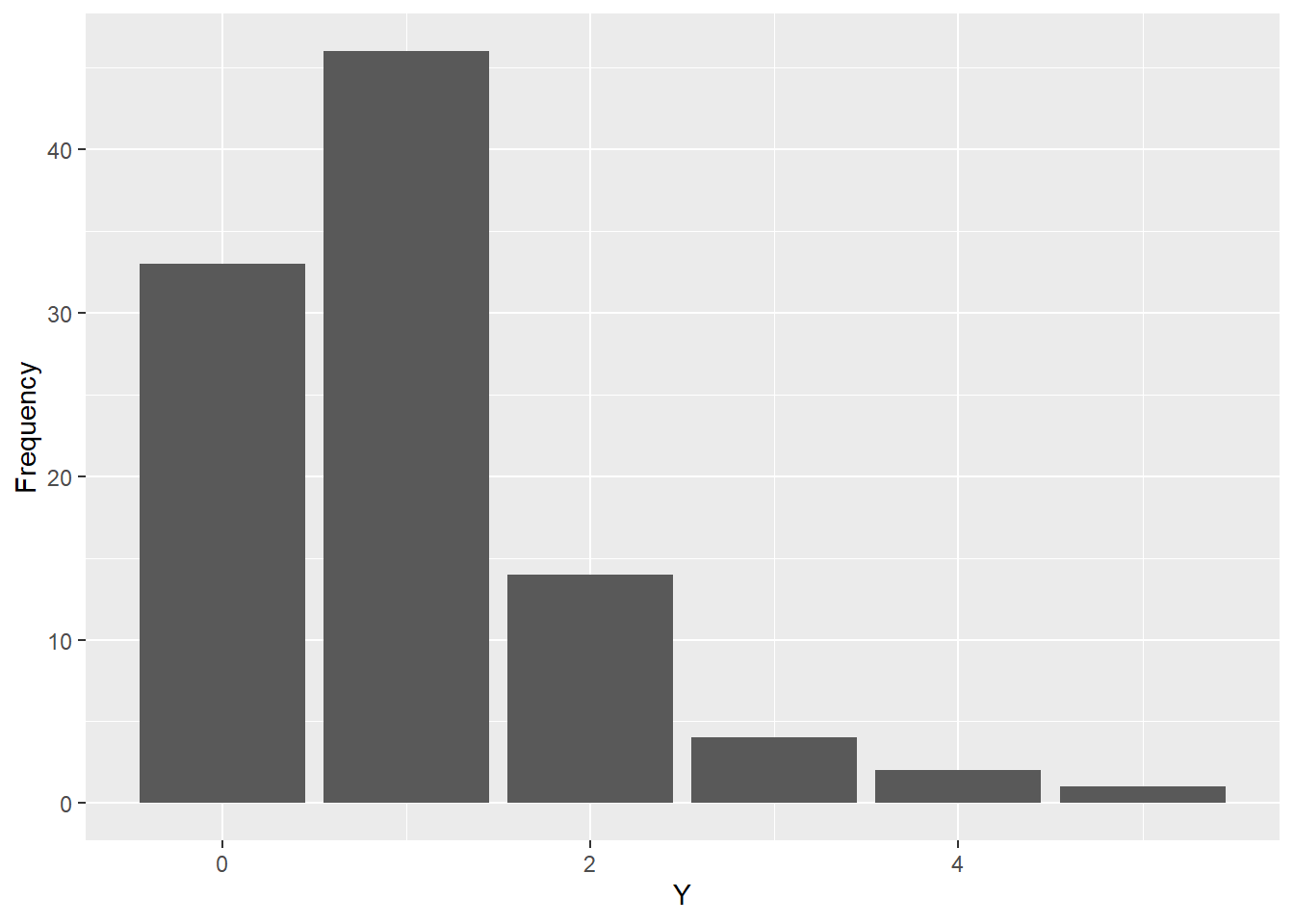
The Poisson model is useful in cases where we have count data. Again, we can model this using a linear model without too many issues in some cases. However, count data usually has a fairly skewed distribution. The below figure provides an example of some simulated count data from a Poisson distribution. As you can see, counts of 0 or 1 occur with the greatest frequency, but higher counts occur with declining regularity.
With data like this you could model it with a linear model, but there’s a chance that you’ll either get fitted values less than 0 (negative counts don’t make sense) or the quality of the fit will start to decline for observations with higher counts. The below figure shows some count data that I simulated which is correlated with a continuous predictor variable. The red line shows a linear regression fit for the data while the blue line shows a Poisson regression fit for the data. The former yields some negative fitted values for smaller count values while it under-estimates expected values for higher counts. The latter doesn’t suffer from this problem.

The process of estimating GLMs in R is very simple and quite similar to what you need to do to estimate a linear model. In base R, in addition to the lm() function there is a glm() function which, as its name suggests, lets you estimate GLMs. With it, you can estimate a wide variety of GLMs, including logit and Poisson models. Let’s try examples of each using some {peacesciencer} data. The below code constructs a leader-year dataset from 1875 to 2010. It then adds information about MIDs, peace spells, leader willingness to use force, and democracy.
## open {peacesciencer}
library(peacesciencer)

## create a leader-year dataset
create_leaderyears(
  standardize = "cow",
  subset_years = 1875:2010
) |>
  ## include details about MIDs
  add_gml_mids() |>
  ## peace spells
  add_spells() |>
  ## leader willingness to use force
  add_lwuf() |>
  ## economic data
  add_sdp_gdp() |>
  ## democracy data
  add_democracy() -> data ## save
With this data, we can estimate a simple logit model of conflict initiation by leaders as a function of their willingness to use force while controlling for quality of democracy, surplus domestic product, and peace spells (number of years for which a country engages in no conflicts). This is what I do in the following code. I use the glm() function, telling it that gmlmidongoing_init is the outcome I’m interested in modeling as a function of theta2_mean (leader willingness to use force), sdpest (natural log of surplus domestic product), and xm_qudsest (quality of democracy). I then tell it the data object in which it should look for these variables and I tell it what kind of GML I want it to estimate using the family option. By telling glm() that I want family = binomial(link = "logit"), it knows I want to model a binary outcome using a logit model. When using the binomial() function, its default is link = "logit", so I could have also just specified family = binomial.
logit_fit <- glm(
  gmlmidongoing_init ~
    theta2_mean +
    sdpest +
    xm_qudsest,
  data = data,
  family = binomial(link = "logit")
)
Just like with lm() where I used summary() to make some statistical inferences about the results of the linear model, I can also use summary() on the output of a GLM:
summary(logit_fit)
Call:
glm(formula = gmlmidongoing_init ~ theta2_mean + sdpest + xm_qudsest,
    family = binomial(link = "logit"), data = data)

Deviance Residuals:
    Min       1Q   Median       3Q      Max
-0.9156  -0.6402  -0.5582  -0.4940   2.5338

Coefficients:
             Estimate Std. Error z value Pr(>|z|)
(Intercept) -2.816760   0.117192 -24.035  < 2e-16 ***
theta2_mean  0.351479   0.033133  10.608  < 2e-16 ***
sdpest       0.054046   0.005038  10.728  < 2e-16 ***
xm_qudsest  -0.158313   0.029367  -5.391 7.01e-08 ***
---
Signif. codes:  0 '***' 0.001 '**' 0.01 '*' 0.05 '.' 0.1 ' ' 1

(Dispersion parameter for binomial family taken to be 1)

    Null deviance: 12626  on 13865  degrees of freedom
Residual deviance: 12315  on 13862  degrees of freedom
  (1104 observations deleted due to missingness)
AIC: 12323

Number of Fisher Scoring iterations: 5
From the results, it’s pretty clear that even when controlling for democracy and surplus domestic product, leader willingness to use force is a statistically significant and positive predictor of whether a country will initiate a fight with other countries. However, one downside of working with GLMs is that the values of the model coefficients can be somewhat unintuitive. With a linear model, the value of the slope is simple. It tells you how much the outcome is expected to change per a one unit change in a predictor. In a logit model, the slope tells you how much the natural log of the odds of an event happening is expected to change per a one unit change in a predictor. What this means in substantive terms is not terribly clear. Furthermore, because the logit model is non-linear when we convert its fitted values to probabilities, the predicted change in the probability of an event given a change in predictor will be different depending on the values of other variables in the data.
For this reason, it’s generally a good idea to visualize some hypothetical predictions from GLMs rather than to just report the raw regression model output. Thankfully, there’s an R package called {sjPlot} that makes it really easy to plot predicted values from many different kinds of models. The below code opens up the package and then uses the function plot_model() to plot the predicted likelihood of conflict initiation given different values of leader willingness to use force (holding all other variables constant at their mean values). Since the function uses ggplot() to construct the figure “under the hood” I can customize it using some {ggplot2} functions after writing +.
library(sjPlot)Warning: package 'sjPlot' was built under R version 4.2.3plot_model(logit_fit, type = "pred", terms = "theta2_mean") +
labs(
x = "Leader Willingness to Use Force",
y = NULL,
title = "Predicted probabilities of MID initiation"
)Data were 'prettified'. Consider using `terms="theta2_mean [all]"` to
get smooth plots.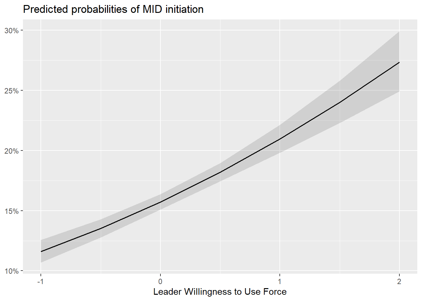
Say we instead wanted to model a count variable like peace spells. This is a count of the number of consecutive years that a country has not started a fight with another country. In this case, we’ll use glm() again, but this time we’ll tell it to estimate a Poisson model. The code looks very similar to that used above. The main differences are that I’ve change the outcome to gmlmidinitspell and I changed the family option to family = poisson.
pois_fit <- glm(
  gmlmidinitspell ~
    theta2_mean +
    sdpest +
    xm_qudsest,
  data = data,
  family = poisson
)
If we use summary() we can, again, report some summary statistics:
summary(pois_fit)
Call:
glm(formula = gmlmidinitspell ~ theta2_mean + sdpest + xm_qudsest,
    family = poisson, data = data)

Deviance Residuals:
    Min       1Q   Median       3Q      Max
-3.3916  -2.2270  -0.9889   0.5185  12.0771

Coefficients:
              Estimate Std. Error z value Pr(>|z|)
(Intercept)  1.2243873  0.0166143  73.695  < 2e-16 ***
theta2_mean -0.1235472  0.0074430 -16.599  < 2e-16 ***
sdpest      -0.0032617  0.0007426  -4.392 1.12e-05 ***
xm_qudsest  -0.2926482  0.0063562 -46.041  < 2e-16 ***
---
Signif. codes:  0 '***' 0.001 '**' 0.01 '*' 0.05 '.' 0.1 ' ' 1

(Dispersion parameter for poisson family taken to be 1)

    Null deviance: 69041  on 13865  degrees of freedom
Residual deviance: 66693  on 13862  degrees of freedom
  (1104 observations deleted due to missingness)
AIC: 93799

Number of Fisher Scoring iterations: 6
Perhaps unsurprisingly, we now see a negative relationship between leader willingness to use force and peace spells. Basically, the more a leader is willing to use force, the fewer consecutive years that country is expected to go without starting a fight. Again, because we’re dealing with a GLM, it’s going to be more intuitive if we plot predicted values rather than try to interpret the model coefficients directly:
plot_model(pois_fit, type = "pred", terms = "theta2_mean") +
  labs(
    x = "Leader Willingness to Use Force",
    y = NULL,
    title = "Expected count of years without MID initiation"
  )
The glm() function will take you pretty far, however there are some other R packages that people have made that offer some advantages. One of my favorites is from the {mfx} package (see documentation here: https://cran.ncc.metu.edu.tr/web/packages/mfx/vignettes/mfxarticle.pdf). One thing that researchers often do when reporting the results from GLMs is show “marginal effects.” Unlike the slopes from GLMs, these do have an intuitive substantive interpretation. For example, for a logit model a marginal effect estimate tells you how much the probability of an event changes per a unit change in a predictor while holding other model variables constant at some meaningful value, such as the mean or median. While marginal effects tend to be conditional, there are still meaningful. However, they can be a pain to calculate. The creator of {mfx} has solved this problem by creating functions that operate very similarly to glm() but which report marginal effects rather than the raw regression slopes.
Here’s an example of the logit analysis the {mfx} way. The final set of estimates reflect the change in the probability of MID initiation per a change in each of the predictors holding everything else at its mean.
## open {mfx}
library(mfx)
Warning: package 'mfx' was built under R version 4.2.3Loading required package: sandwichLoading required package: lmtestLoading required package: zoo
Attaching package: 'zoo'The following objects are masked from 'package:base':
as.Date, as.Date.numericLoading required package: MASSWarning: package 'MASS' was built under R version 4.2.3
Attaching package: 'MASS'The following object is masked from 'package:dplyr':
selectLoading required package: betaregWarning: package 'betareg' was built under R version 4.2.3## estimate the model using logitmfx()
mfx_logit <- logitmfx(
gmlmidongoing_init ~
theta2_mean +
sdpest +
xm_qudsest,
data = data
)
mfx_logit ## show outputCall:
logitmfx(formula = gmlmidongoing_init ~ theta2_mean + sdpest +
xm_qudsest, data = data)
Marginal Effects:
dF/dx Std. Err. z P>|z|
theta2_mean 0.0476237 0.0044506 10.7005 < 2.2e-16 ***
sdpest 0.0073230 0.0006650 11.0121 < 2.2e-16 ***
xm_qudsest -0.0214506 0.0039640 -5.4114 6.254e-08 ***
---
Signif. codes: 0 '***' 0.001 '**' 0.01 '*' 0.05 '.' 0.1 ' ' 1If you compare this output to the summary of the original logit model fit, you can see that while the results tell a similar story in terms of statistical significance and the direction of relationships, the numerical values are different:
summary(logit_fit)
Call:
glm(formula = gmlmidongoing_init ~ theta2_mean + sdpest + xm_qudsest,
    family = binomial(link = "logit"), data = data)

Deviance Residuals:
    Min       1Q   Median       3Q      Max
-0.9156  -0.6402  -0.5582  -0.4940   2.5338

Coefficients:
             Estimate Std. Error z value Pr(>|z|)
(Intercept) -2.816760   0.117192 -24.035  < 2e-16 ***
theta2_mean  0.351479   0.033133  10.608  < 2e-16 ***
sdpest       0.054046   0.005038  10.728  < 2e-16 ***
xm_qudsest  -0.158313   0.029367  -5.391 7.01e-08 ***
---
Signif. codes:  0 '***' 0.001 '**' 0.01 '*' 0.05 '.' 0.1 ' ' 1

(Dispersion parameter for binomial family taken to be 1)

    Null deviance: 12626  on 13865  degrees of freedom
Residual deviance: 12315  on 13862  degrees of freedom
  (1104 observations deleted due to missingness)
AIC: 12323

Number of Fisher Scoring iterations: 5
The {mfx} logit function by default shows the marginal effect for the mean of the data, but you can turn this option off and instead have the function return the average of the marginal effects by writing atmean = FALSE. This is more computationally intensive, so it’s generally best to go with the default.
{mfx} also has a function for estimating a Poisson model. Unlike the output with the glm() version of the model, poissonmfx() returns the expected change in the count of peace years per a change in each of the model predictors.
mfx_pois <- poissonmfx(
  gmlmidinitspell ~
    theta2_mean +
    sdpest +
    xm_qudsest,
  data = data,
)
mfx_pois
Call:
poissonmfx(formula = gmlmidinitspell ~ theta2_mean + sdpest +
xm_qudsest, data = data)
Marginal Effects:
dF/dx Std. Err. z P>|z|
theta2_mean -0.3510235 0.0210922 -16.6423 < 2.2e-16 ***
sdpest -0.0092670 0.0021094 -4.3932 1.117e-05 ***
xm_qudsest -0.8314747 0.0175925 -47.2631 < 2.2e-16 ***
---
Signif. codes: 0 '***' 0.001 '**' 0.01 '*' 0.05 '.' 0.1 ' ' 1Another feature with {mfx} is that you can specify that you want to calculate what are called robust standard errors. You can also choose to cluster the standard errors by one or two grouping variables in the data. Using robust standard errors is generally a good idea when working with observational data because classical standard errors often assume the data do not deviate from core model assumptions about the variance of the outcome. This rarely is the case, and as a result classical standard errors are too optimistic. In the case of the logit and Poisson regression analyses above, it would be advisable to calculate robust standard errors and cluster them by leader ID. Here’s a version of the logit model estimated above, but this time with the options robust = TRUE and clustervar1 = "leader".
mfx_logit_rob <- logitmfx(
  gmlmidongoing_init ~
    theta2_mean +
    sdpest +
    xm_qudsest,
  data = data,
  robust = T,
  clustervar1 = "leader"
)
So that it’s easier to see the difference this makes, in the below code I make a regression table using {texreg}. As you can see, the robust-clustered standard errors are about double the size of the classical standard errors.
library(texreg)Version: 1.38.6
Date: 2022-04-06
Author: Philip Leifeld (University of Essex)
Consider submitting praise using the praise or praise_interactive functions.
Please cite the JSS article in your publications -- see citation("texreg").
Attaching package: 'texreg'The following object is masked from 'package:tidyr':
extractscreenreg(
list(
"Classic SEs" = mfx_logit,
"Clustered SEs" = mfx_logit_rob
),
digits = 3
)
============================================
                Classic SEs    Clustered SEs
--------------------------------------------
theta2_mean         0.048 ***      0.048 ***
                   (0.004)        (0.009)
sdpest              0.007 ***      0.007 ***
                   (0.001)        (0.002)
xm_qudsest         -0.021 ***     -0.021 *
                   (0.004)        (0.008)
--------------------------------------------
Num. obs.       13866          13866
Log Likelihood  -6157.585      -6157.585
Deviance        12315.170      12315.170
AIC             12323.170      12323.170
BIC             12353.319      12353.319
============================================
*** p < 0.001; ** p < 0.01; * p < 0.05
6.3 A note of caution
Now that I’ve equipped you with some tools for data analysis with conflict data, I’ve probably given you just enough to be dangerous. Be careful in your use of logit and Poisson models and your selection of predictor variables. You’ll quickly find that the inclusion and exclusion of certain variables in your regression models may either make or break your expectations about relationships in the data. You’ll face the temptation to only report the results from models that support your claims, while you’ll try and pretend that less favorable specifications don’t exist.
I understand this temptation, and I’ve fallen pray to it before. The best way to hold yourself accountable is to come up with an analysis plan before you actually get your hands on the data. Such Pre-analysis Plans or PAPs are often used in the context of randomized controlled trials. There’s a movement in favor of using them for observational studies as well, but this is easier said than done. Even so, the more planning you can do before seeing your data (and documentation you can provide that you in fact made your plans without seeing the data), the better and more trustworthy your results will be, especially if you want to make strong causal claims with your data.
Such an approach does not mean that you can’t engage in exploratory data analysis. Often times when we get our hands on some data, we realize that our initial plans need some revision. You can actually build this flexibility into your plans. The key is to add a proviso that additional exploratory analysis is just that—exploratory—and that any conclusions drawn are suggestive but not confirmatory. While the conclusions you draw from this kind of analysis are weaker, they can serve as a jumping off point for future research, generating to questions and motivating new ideas for theory generation and testing.
Much of the research that we do in the coming chapters will be exploratory in nature. While we won’t be looking to confirm or reject any claims made by Blattman (2023) in Why We Fight, we will draw some suggestive inferences that either support or conflict with parts of Blattman’s argument. Without further ado, let’s get to it.
6.4 Additional resources on regression models
You might find the following resources helpful if you want to go deeper with statistical modelling in R:
I might teach you just enough to be dangerous. That’s not my intention, but…↩︎