10  Uncertainty

Blattman (2023) argues that uncertainty leads to war for a number of reasons:

• It creates incentives to signal power and resolve, creating the need to engage in costly and risky behaviors.

• It creates a need for sides to engage in low-level disputes or skirmishes so that beliefs about each side’s power converge.

• It creates incentives to bluff, forcing the other side to make a hard choice: accept a bargain that might lead them to give up less than they deserve or call the bluff and risk a costly war and discover the other side was telling the truth about their power.

Blattman (2023) points to several real-world examples of uncertainty in action. One of the most prominent was the US decision to invade Iraq in 2003. Though factors other than uncertainty were also at work, Saddam had lots of incentives to bluff about Iraq’s strength—particularly with respect to its stockpile of Weapons of Mass Destruction (WMD).

However, as compelling the argument for uncertainty as a cause of war is, looking at a handful of examples isn’t enough to systematically demonstrate uncertainty’s influence. So, in this chapter we’ll look at some conflict data with {peacesciencer} to see if we can infer the role of uncertainty in a more rigorous way.

10.1 Hypotheses to test

The first thing we need to consider is what patterns we expect to see in the world that we can capture with data, if uncertainty is actually a reason for war. There are many different predictions that follow from Blattman’s argument. Let’s focus on just two:

Hypothesis 1: Low-level skirmishes can help sides improve their information about the power of rivals, so we should observe that the greatest number of conflicts are small scale and short in duration.

Hypothesis 2: The presence of many rivals can create incentives to signal power and resolve, so when a country has many rivals, it should be more apt to initiate conflicts.

Thankfully, we can test both of these claims using datasets constructed with {peacesciencer}. For the first, we’ll look at conflict-level data. This is a level of analysis that we haven’t considered so far, because generally we’ve been interested in examining the effects of leader characteristics or specific conditions within countries that might correspond with reasons for war. However, hypothesis 1 points to a simple descriptive reality: that most conflicts are small-scale. To test this claim, all we need to do is look at conflicts themselves rather than details about the actors involved.

For the second hypothesis, we’ll create a country-year dataset and use counts of the number of strategic rivalries a country has to see whether more rivalries increases the likelihood that a country initiates militarized interstate disputes (MIDs) with other countries.

10.2 Data

First, we’ll get our R environment set up. The below code opens the {tidyverse} and {peacesciencer}. It also opens up the {coolorrr} package, which is an R package that I created to make working with custom color palettes easier.

## open usual packages
library(tidyverse)
library(peacesciencer)

## open {coolorrr} and use set_theme() and set_palette()
## to customize data viz appearance and color palettes
library(coolorrr)
set_theme()
set_palette()

First we need some conflict-level data. In addition to providing tools for creating datasets, {peacesciencer} also gives you access to many pre-existing datasets that are already populated with variables. One of these is called gml_mid_disps, which is a collapsed and pared down conflict-level dataset. Each observation in the data is a unique MID and each column provides some details about each MID, like its fatality level, duration, and so on.

The below code opens the {socsci} package, which is helpful for making some changes to our data prior to analysis. The raw data has all the variables we need, but some need to be re-coded so that it’s clear what different numerical values mean. For example, the entries for hostlev and fatality are numerical codes that correspond with specific substantive categories. The below code adds some new columns to the data that more faithfully reflect what these values mean. From hostlev, I make a column called all_out_war which takes the value of “War” if hostlev == 5, “Low-level Dispute” otherwise. I also, map fatality codes to a set of labels that indicate what range of fatalities was observed for each MID. I then save the updated version of the data as an object called mid_data.

library(socsci) ## for coding ordered categories

Loading required package: rlang

Warning: package 'rlang' was built under R version 4.2.3

Attaching package: 'rlang'

The following objects are masked from 'package:purrr':

    %@%, flatten, flatten_chr, flatten_dbl, flatten_int, flatten_lgl,
    flatten_raw, invoke, splice

Loading required package: scales

Attaching package: 'scales'

The following object is masked from 'package:purrr':

    discard

The following object is masked from 'package:readr':

    col_factor

Loading required package: broom

Warning: package 'broom' was built under R version 4.2.3

Loading required package: glue

gml_mid_disps |>
  mutate(
    
    ## is the conflict an all-out war?
    all_out_war = 
      ifelse(hostlev == 5, "War", "Low-level Dispute"),
    
    ## fatalities
    fatality_cat = frcode(
      fatality == 0 ~ "0",
      fatality == 1 ~ "1-25",
      fatality == 2 ~ "26-100",
      fatality == 3 ~ "101-250",
      fatality == 4 ~ "251-500",
      fatality == 5 ~ "501-999",
      fatality == 6 ~ "1,000 +",
      TRUE ~ "Unknown"
    )
  ) -> mid_data

We also need some data to explore the impact of rivalries on conflict initiation. This is more straightforward to do. The below code creates a state-year dataset and then populates it with MID initiation data, peace spells, and details about the number of different strategic rivalries a country has with others in the international system. The code saves the data as an object called rivals_data.

create_stateyears() |>
  add_gml_mids() |>
  add_spells() |>
  add_strategic_rivalries() -> rivals_data

Joining with `by = join_by(ccode, year)`

Warning in xtfrm.data.frame(x): cannot xtfrm data frames

Joining with `by = join_by(orig_order)`

Warning in xtfrm.data.frame(x): cannot xtfrm data frames

Joining with `by = join_by(orig_order)`
Joining with `by = join_by(ccode, year)`

10.3 Analysis

10.3.1 Are Most Conflicts Small-scale?

With the mid_data object we can assess the distribution of conflict sizes using three factors:

1. Whether the hostility level escalated to that of an all-out war.
2. The fatality level of conflicts.
3. The duration of conflicts.

Hypothesis 1 tells us that we should expect most conflicts to be small scale. So that means most MIDs in the data shouldn’t be all-out wars, they should have low fatality levels, and they should last a short amount of time. We’ll tackle these in order.

The below data visualization helps us to determine whether all-out wars are relatively uncommon among the full set of MIDs that we observe in the data. The below code breaks the data down by decades, and then for each it decade calculates the share of MIDs that are not all-out wars relative to the share that are. It then reports the results in a stacked bar chart using colors to highlight which calculations are for which kind of conflict. It’s pretty clear that most MIDs fail to reach the level of all-out war. At the most extreme, nearly a quarter of MIDs in a decade rose to the level of war, while in many decades the rate is much smaller.

## show distribution of conflict types
library(shadowtext)

Warning: package 'shadowtext' was built under R version 4.2.3

mid_data |>
  mutate(
    decade = floor(styear / 10) * 10
  ) |>
  group_by(decade) |>
  ct(all_out_war) |>
  ggplot() +
  aes(
    x = decade,
    y = pct,
    fill = all_out_war
  ) +
  geom_col() +
  geom_shadowtext(
    data = . %>% filter(all_out_war == "War" & pct > 0),
    aes(label = paste0(round(100 * pct), "%")),
    color = "white",
    fontface = 4,
    vjust = -0.2
  ) +
  labs(
    x = NULL,
    y = NULL,
    title = "% of New Conflicts per Decade by Type",
    fill = NULL
  ) +
  scale_x_continuous(
    breaks = seq(1810, 2010, by = 10)
  ) +
  scale_y_continuous(
    labels = scales::percent
  ) +
  theme(
    axis.text.x = element_text(
      angle = 45,
      hjust = 1
    ),
    legend.position = "bottom"
  ) +
  ggpal(aes = "fill")

Do we see a similar pattern when we look at conflict fatalities? It turns out that we do. The below code calculates for a given decade the share of conflicts that fall into different fatality level ranges. Across decades, a majority (or at minimum a plurality) of MIDs result in 0 battle-related deaths. Only a very small number result in more than 1,000 total battle-related deaths.

## show distribution of conflict fatalities
mid_data |>
  mutate(
    decade = floor(styear / 10) * 10
  ) |>
  filter(fatality_cat != "Unknown") |>
  group_by(decade) |>
  ct(fatality_cat) |>
  ggplot() +
  aes(
    x = decade,
    y = pct,
    fill = fatality_cat
  ) +
  geom_col(
    color = "black"
  ) +
  labs(
    x = NULL,
    y = NULL,
    title = "Distribution of Conflict Fatality Levels",
    fill = NULL
  ) +
  scale_x_continuous(
    breaks = seq(1810, 2010, by = 10)
  ) +
  scale_y_continuous(
    labels = scales::percent
  ) +
  theme(
    axis.text.x = element_text(
      angle = 45,
      hjust = 1
    ),
    legend.position = "bottom"
  ) +
  ggpal(
    type = "sequential",
    aes = "fill",
    ordinal = T,
    levels = 7
  )

Finally, what about conflict duration? Is it the case that most conflicts are short-lived? The answer is yes. The below code uses a kind of plot called a “ridge” plot to summarize the probability distribution of conflict duration in days by decade in the data. A dashed line is used at the 365 day mark to note when values go beyond a year in duration. As is clear, most conflicts are much shorter in duration than a year. Conflicts that last a year or more are incredibly rare.

## show distribution of conflict fatalities
library(ggridges)
mid_data |>
  mutate(
    decade = as.factor(floor(styear / 10) * 10)
  ) |>
  ggplot() +
  aes(
    x = maxdur, 
    y = decade,
    fill = as.numeric(decade)
  ) +
  geom_vline(
    xintercept = 365,
    linetype = 2
  ) +
  annotate(
    "text",
    x = 365,
    y = "1810",
    label = "1 Year",
    hjust = -0.2
  ) +
  geom_density_ridges(show.legend = F) +
  labs(
    x = NULL,
    y = NULL,
    title = "Distribution of Conflict Duration in Days"
  ) +
  ggpal("sequential", "fill") +
  scale_x_continuous(
    labels = scales::comma
  )

Picking joint bandwidth of 50.2

Taken together, these patterns are consistent with hypothesis 1. Now, let’s shift gears and consider hypothesis 2.

10.3.2 Do rivalries drive conflict?

Hypothesis 2 holds that the existence of many rivals can exacerbate the problem of uncertainty. Because an actor knows that its actions matter not only in their interaction with an opponent but also for all possible future interactions with other opponents, having many rivals to contend with can create incentives to signal strength and resolve. One unfortunate consequence of this is an increased likelihood of starting fights with other countries as a way of sending costly signals of military power and willingness to use it. Using the country-year dataset we constructed above, we can see whether this is evident in the data.

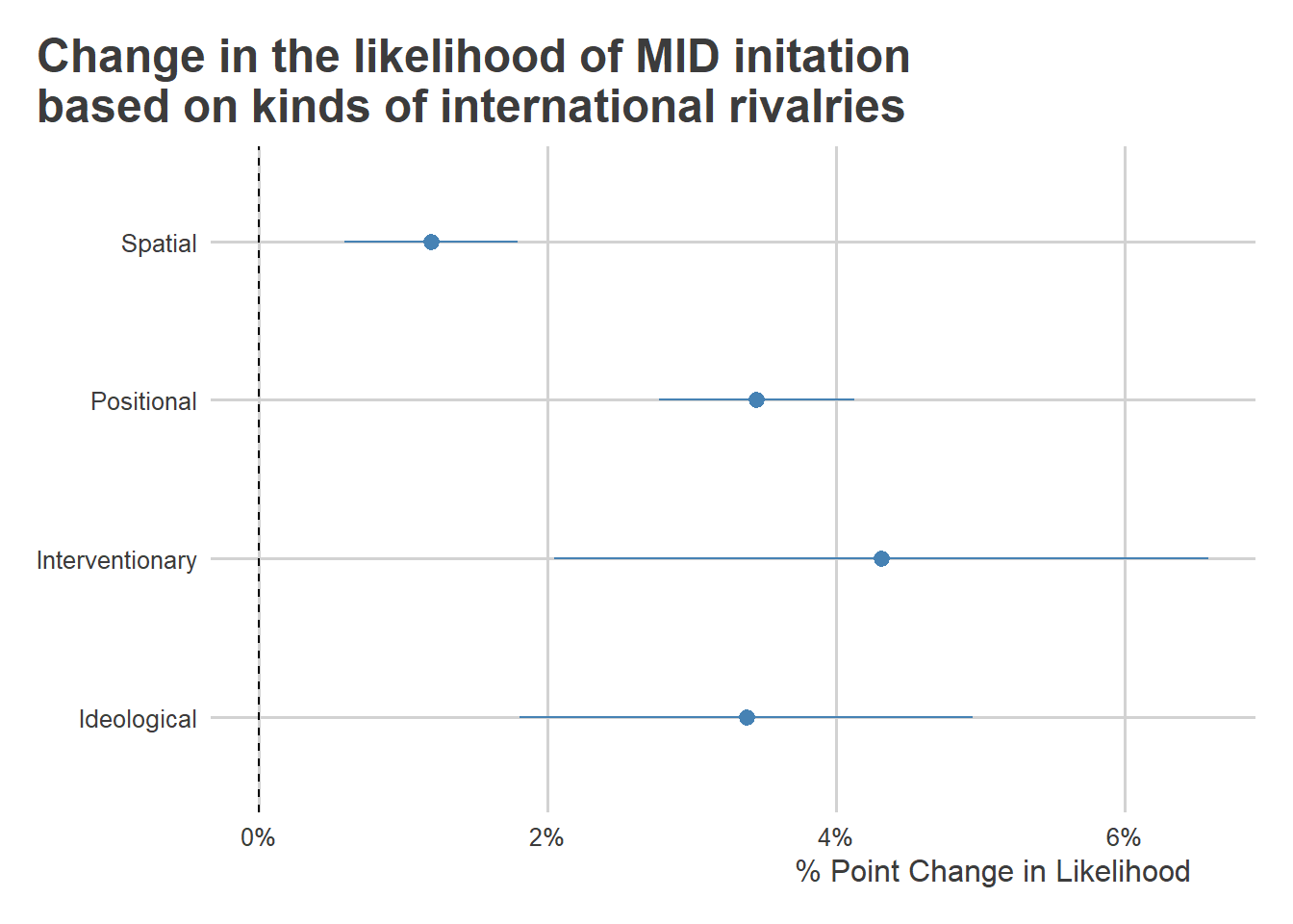
In the below code, I have R estimate a logit regression model using yearly counts of four different kinds of strategic rivalries a country has with other countries in the international system. In the model I control for a cubic peace spells trend. I have R summarize the results in a coefficient plot that reports the marginal effects of the different rivalry types with 95% confidence intervals. The estimates tell us how, all else equal, adding one extra kind of rival changes the probability that a country initiates a militarized dispute with another country in a given year. Each of the four types of rivalries has a positive correlation with MID initiation. Given how rare conflict is in general, the size of the estimates are quite substantial. Moreover, they’re statistically significant and positive, consistent with hypothesis 2.

## open {mfx} package
library(mfx)

## estimate logit model with robust-clustered standard errors
logitmfx(
  gmlmidonset_init ~ ideological +
    interventionary + positional + spatial +
    gmlmidinitspell + I(gmlmidinitspell^2) + 
    I(gmlmidinitspell^3),
  data = rivals_data,
  robust = T,
  clustervar1 = "ccode"
) -> model_fit

## summarize the results in a coefficient plot
model_fit |>
  broom::tidy() |>
  filter(
    !str_detect(term, "gml")
  ) |>
  mutate(
    lo = estimate - 1.96 * std.error,
    hi = estimate + 1.96 * std.error
  ) |>
  ggplot() +
  aes(x = estimate, xmin = lo, xmax = hi, y = term) +
  geom_pointrange(
    color = "steelblue"
  ) +
  geom_vline(
    xintercept = 0,
    linetype = 2
  ) +
  labs(
    x = "% Point Change in Likelihood",
    y = NULL,
    title = "Change in the likelihood of MID initation\nbased on kinds of international rivalries"
  ) +
  scale_x_continuous(
    labels = scales::percent
  ) + 
  scale_y_discrete(
    labels = c(
      "Ideological",
      "Interventionary",
      "Positional",
      "Spatial"
    )
  )

10.4 Conclusion

Uncertainty can be a potent cause of war, and it even can be the reason why we see countries engage in low-level skirmishes with each other. While the above analysis does not confirm the role of uncertainty as a reason for war, the results are consistent with the argument Blattman (2023) makes about uncertainty’s implications. In the next chapter, we’ll turn our attention to yet another reason for war—commitment problems.

Blattman, Christopher. 2023. Why We Fight: The Roots of War and the Paths to Peace. Penguin.