library(tidyverse)
dt <- read_csv("https://raw.githubusercontent.com/milesdwilliams15/Teaching/refs/heads/main/DPR%20201/Data/dpr201_unit1_data.csv")4 Modeling Data
4.1 Goals
Learning objectives:
Understand the basics of linear regression.
Learn how to estimate a regression model in R and interpret the output.
4.2 What is a model?
When someone says that they’ve developed a statistical model of some event or behavior, this often evokes a sense of mysticism and technical prowess to the uninitiated. In this chapter, I want to make the process of data modeling accessible. There’s nothing mystical about data models, and you’d be surprised how little technical prowess it takes to estimate one. If you have some data and some good intuitions, data modeling really just boils down to knowing the right code to get your computer to do the heavy lifting for you. And if you want to do something really dangerously easy, many LLMs not only can write, but also run analysis code for you. If you don’t have some basic knowledge and skills already in place, you can do some real damage.
Even with some background in statistics and modeling, there are many misconceptions and plain wrong instructions, explanations, and interpretations of even common models online. Without the proper understanding to inform your analysis and modeling choices, you run the risk of using models in an inappropriate way.
Different models make different assumptions. Some make many assumptions, while others make few. Some models were designed to be general purpose tools that are applicable across a wide range of data, while others were developed to solve a particular problem unique to a certain data type.
In this class, we’re going to focus our attention on the linear regression model. As I’ll discuss more in the next section, the linear model is quite general because, despite its name, it can be made nonlinear and more flexible in a variety of ways. And as we’ll discuss more in the next chapter, the linear model makes minimal or no assumptions that bear on our ability to do statistical inference (that is, to quantify the role of chance in our data).
Before getting to that, I want to first give you a brief outline of a data model that can generalize to a wide variety of model types. To do this I’m going to introduce some basic mathematical notation, so bear with me.
First, let \(y_i\) represent an outcome variable that we want to model using some explanatory variable, \(x_i\). The subscript \(i\) is a convention that is often used to signal that \(x\) and \(y\) are variables for which we observe unique instances. The letter \(i\) is a stand-in for any integer from \(1, ..., n\) where \(n\) is the total number of observations in a dataset.
We can represent a model of \(y_i\) given \(x_i\) by writing:
\[ y_i = f(x_i; \theta) \]
The \(f(\cdot)\) is a stand-in for some arbitrary function that defines how values of \(x_i\) get mapped to values of \(y_i\), and \(\theta\) is a set of parameters that inform this mapping. This formulation can be read to mean that \(y_i\) is a function of \(x_i\), given \(\theta\).
Now, a model is pretty useless if we don’t have a way to fit the model to actual data. Depending on the context, the process of model fitting might also be called model training or even learning. Models are fit using a rule (criterion) that specifies what a good fit looks like. Usually this means an objective function that we must try to optimize. Such a function could look something like this:
\[ g(y_i, x_i; \theta) = \sum_{i = 1}^n [y_i - f(x_i; \theta)]^2 \]
The above is a quadratic equation that measures the sum of the squared differences between observed values of the outcome variable and predicted/fitted values spit out by the model. The goal is to find values of the model parameters (the \(\theta\)s) that make this sum as small as possible, because if the sum is small, that means there’s little difference between reality and the model’s predictions.
Once we’ve done this process, which usually involves some multidimensional calculus or a computer algorithm, we then are left with a set of estimates for the \(\theta\) parameters. These are denoted as \(\hat \theta\) (pronounced “theta hat”). With them in hand, we now have a fitted model for the data.
If you’re feeling lost right about now, keep hanging on. I think this abstract introduction will make more sense when we apply it to linear regression. The main takeaways that I want to emphasize are:
- Models are ways of representing the relationship between an outcome variable and one or more explanatory variables.
- Models usually have parameters that we need to estimate to fit the model to data.
- To estimate these parameters, we need an objective function which gives us a rule or benchmark to know which parameter values give us the best fit.
4.3 The basics of linear regression models
Let’s get rid of \(f(\cdot)\). It’s pretty abstract and doesn’t tell us any thing specific about how we’re going to model some data. Instead, let’s talk about the linear regression model. We sometimes just call this a linear model or linear regression.
Using the same variables as before, we can write out a linear model like so:
\[ y_i = \beta_0 + \beta_1 x_i + \epsilon_i \]
If you’ve taken linear algebra before, this formula should look familiar. Do you recall the formula \(y = mx + b\)? The linear model is a version of this really simple equation. \(\beta_0\) is the intercept, which is the value of \(y_i\) when \(x_i\) is zero. \(\beta_1\) is the slope, which indicates the “rise over the run,” or how the expected value of \(y_i\) changes as \(x_i\) changes. Finally, \(\epsilon_i\) represents random noise, which is variation in \(y_i\) that isn’t explained by \(x_i\). We also call this the “error term.”
When there is just one explanatory variable in a linear model, we sometimes call it a “simple” linear regression model. But when we add more than one explanatory variable, we instead call it a “multiple” regression model.
You’ll sometimes see people mistakenly use the term “multivariate” regression model to describe the same thing. This isn’t what the term “multivariate” means. Multivariate regression refers to a kind of model where there are multiple outcome variables rather than multiple explanatory variables. You have to be careful with your terms, because a mistake like that can signal to others that you don’t know what you’re talking about (useful to know for future job interviews).
Speaking of multple regression, here’s an example of one that includes two explanatory variables (\(x_i\) and now a new one called \(z_i\)):
\[ y_i = \beta_0 + \beta_1 x_i + \beta_2 z_i + \epsilon_i \]
There’s really no limit (in theory) for how many explanatory variables you can include, but there are plenty of practical reasons to be choosy about how many, and which, to add to the model.
Speaking of things to keep in mind, before we talk about fitting linear models to data, I mentioned earlier that all models make assumptions. Linear regression is no exception. If you’re using a linear model, you need to assume that two things are true:
- Data validity: Your data is relevant for your research and is reliable.
- Additivity and linearity: The basic mathematical assumption of linear regression is that the outcome is a linear function of separate explanatory variables.
Data validity should be obvious, but too often people forget that your model is only as good as your data. If you have bad data, you’ll have a bad model. Put another way: garbage in, garbage out.
Additivity and linearity are also important, but in practice there actually is no way to know for sure that these assumptions are “correct.” In fact, they probably aren’t. But this is no big deal. We really just care about whether these assumptions are useful. Is it good enough to assume additivity and linearity?
Now, some people impose additional assumptions on linear models, but these actually don’t matter as much as you’d think. Typical extra assumptions include things like:
- Independence of errors: The error term (\(\epsilon_i\)) should be independently distributed (one observation’s outcome should not depend on the outcome of others).
- Equal variance of errors: The error term should not be “heteroskedastic” (a fancy term that means the variance for some observations is different than for others).
- Normality of errors: The error term should follow a normal distribution.
These assumptions all deal with the error term in the model, but they’re of secondary importance because they don’t actually have much bearing on the estimation of linear model parameters. They do matter for statistical inference, but as we’ll discuss in the next chapter it’s easy enough to deal with violations of these assumptions without doing anything drastic.
I also should note that there aren’t very reliable ways to check whether these secondary assumptions are violated; though, in many introductory stats courses the suggestion is made that you can do things like plot model residuals (these are estimates of the model error term) to determine if these assumptions aren’t met. This is actually very bad advice if your main goal is statistical inference. Most violations of these assumptions aren’t visible to the naked eye. For example, you can have heteroskedasticity of unknown form (that sounds like a terrible disease), and it won’t show up in a residual plot. And even if things look off, that doesn’t mean that the model estimates are biased (prone to error in one way or the other). Often the estimates are just fine. So, if you hear someone tell you to check model residuals, just say “no.” I offer this warning because of personal experience: I got scolded (severely) by one of my statistical methods professors in grad school for plotting residuals, which left a lasting impression on me. I’d like to save you from making the same mistake.
4.4 OLS and the building blocks of linear model estimation
Now that we have a model, we need a way to fit it to some data. I previously noted that we need an objective function to do this. For linear regression, the standard approach is to use a method called ordinary least squares (OLS). The OLS objective function for a linear model looks something like this:
\[ \text{SSR} = \sum_{i = 1}^n (y_i - \beta_0 - \beta_1 x_i - \beta_2 z_i)^2 \]
We call this the sum of the squared residuals. It’s the sum of the squared differences between the outcome variable we want to model and its fitted values produced by the linear model. (Hey! That sounds just like the hypothetical objective function I talked about earlier. It’s almost like I’m trying to teach you something.)
To simplify this function, we can represent the linear model fit for the data by writing:
\[\hat y_i = \beta_0 + \beta_1 x_i + \beta_2 z_i\]
Notice that the \(\epsilon_i\) term is gone and that there’s a \(\hat \cdot\) symbol above the outcome variable. This signifies that we’re talking about fitted or predicted values of the outcome rather than observed values.
By substituting \(\hat y_i\) for \(y_i\), the SSR equation looks like this:
\[\text{SSR} = \sum_{i = 1}^N (y_i - \hat y_i)^2\]
FYI, the differences between observed and estimated values of the outcome variable are also referred to as residuals. Residuals are essentially our estimate of the error term, and to help clarify when we’re referring to residuals rather than the error, we use the hat symbol again. For example:
\[\hat \epsilon_i = y_i - \hat y_i\]
If we substitute this into the SSR equation, we can clearly see why it’s called the sum of the squared residuals:
\[\text{SSR} = \sum_{i = 1}^N \hat \epsilon_i^2\]
Now that we have an objective function, there’s just one more thing we need (aside from data). We need an estimator, which is a rule for calculating a quantity of interest.
I know what you’re thinking. You thought the objective function was the rule. Yes and no. It’s a rule in the sense that it gives us a way to measure how well a model performs. But it doesn’t tell us how to find the best possible model. This is where an estimator comes in. An estimator is a rule for finding the best estimate given an objective function.
For the OLS method, the estimator is the solution for the \(\beta\) values that minimize the SSR equation. We want to minimize the SSR because the smaller the differences between the observed values of the outcome variable and the estimated values from the model, the better the model is doing.
The cool think about OLS (okay, you may not think it’s cool, but I do) is that mathematicians long, long ago found the formula for estimating linear regression parameters using OLS by way of some simple multivariate calculus (alright, I get it, multivariate calculus doesn’t sound cool or simple).
Here’s why you should be happy about this. The fact that they found this solution means that estimating linear models is just a plug-and-chug process of number crunching. In fact, you can actually estimate a linear model by hand using a pencil and paper (which I was forced to do in grad school). Don’t worry, I won’t make you do that, because R can do that for you.
I do want to show you the solution, though. Say you just had a simple linear regression model with one explanatory variable. You can find the slope for this explanatory variable by calculating:
\[\hat \beta_1 = \frac{\sum_{i = 1}^N (y_i - \bar y) (x_i - \bar x)}{\sum_{i = 1}^N (x_i - \bar x)^2}\]
The “bar” over \(x\) and \(y\) represents the mean. So \(\bar x\) is the mean of \(x_i\) and \(\bar y\) is the mean of \(y_i\).
Once you have \(\hat \beta_1\), you can find the intercept by calculating:
\[\hat \beta_0 = \bar y - \hat \beta_1 \bar x\]
The math becomes a bit more involved when we start talking about multiple regression models with more than one explanatory variable. But the idea remains the same.
Another cool thing about the OLS estimator (there I go using “cool” again) is that it is based on textbook, dare I say basic, statistical calculations. If you can calculate things like means, variance, covariance, and standard deviation, you have all that you need for linear regression.
The mean is pretty straightforward. Say you wanted the mean of \(x_i\). You’d just need to take the sum of all the values of \(x_i\) and then divide by the total number of observations in the data.
\[\bar x = \frac{\sum_{i=1}^Nx_i}{N}\]
The variance of \(x_i\) relies on already having the mean calculated, and it’s calculated like so:
\[var(x_i) = \frac{(x_i - \bar x)^2}{N - 1}\]
We divide by \(N - 1\) since we already used all of \(N\) to calculate the mean. You lose a degree of freedom by going a step further to calculate the variance.
The standard deviation is then just the square root of the variance:
\[\sigma_x = \sqrt{var(x_i)}\]
The standard deviation is a measure of the average variation in a variable around its mean. For example, a standard deviation of 2 means that, on average, the typical value of \(x_i\) lies 2 units above or below the mean of \(x_i\).
Finally, there’s a version of variance known as covariance. Instead of capturing the variation in a single variable, it’s a way of capturing how two variables covary (hence the name). It’s calculated as:
\[cov(y_i, x_i) = \frac{\sum_{i = 1}^N(y_i - \bar y)(x_i - \bar x)}{N - 1}\]
Unlike variance, covariance can be positive or negative. If the covariance is positive, that means the variables are positively correlated: as one goes up, the other does, too. If the covariance is negative, that means the variables are negatively correlated: as one goes up, the other goes down.
I mentioned that these calculations are the basic building blocks of the OLS estimator. Here’s how. You already know that the mean is part of the solution, but what you might not realize is that the variance and covariance are, too. Remember the equation for the slope parameter for the simple linear regression model? That solution is mathematically equivalent to this:
\[\hat \beta = \frac{cov(y_i, x_i)}{var(x_i)}\]
If you don’t believe me, note that both the covariance and variance are divided by \(N - 1\). Since these are both in the numerator and denominator, they cancel out, leaving you with the solution I showed you earlier.
But wait, there’s more! I should also mention that another statistic that you need to know about is constructed on these same building blocks as well. Have you heard of Pearson’s correlation coefficient, also known as \(\rho\) (“rho”)?
\(\rho\) is closely related to the slope parameter from a linear regression model, but it is meant to quantify something slightly different. While \(\beta_1\) tells us how much \(y_i\) is expected to increase per an increase in \(x_i\), \(\rho\) tells us the relative strength of this linear relationship. It can take values between -1 and 1 where 1 means that two variables have a perfectly linear positive relationship while -1 means they have a perfectly linear negative relationship. 0 means that they have no linear relationship at all.
\(\rho\) is calculated as follows:
\[\hat \rho = \frac{cov(y_i, x_i)}{\sigma_y \sigma_x}\]
Like the OLS estimator, the numerator is the covariance of two variables. But instead of dividing this by the variance of the explanatory variable, it’s divided by the product of the standard deviation of each variable. This solution is what ensures that \(\rho\) stays between the bounds (inclusive) of -1 and 1.
4.5 Estimating linear models with R
Everything I’ve talked about so far has been theoretical and abstract. In this section I want to walk you through some applied examples using the U.S. foreign aid dataset introduced in the last chapter.
I noted earlier that model fitting is a trivial thing to do with statistical software. Your computer will take care of all the calculations discussed in the last section. All you have to do is use R to tell your computer to do it.
R is, first and foremost, tailored for statistical programming. That means the code for doing linear regression in R is pretty straightforward. The workhorse function for linear models in R is lm(), which stands for “linear model.” Here’s how you use it.
First, we need some data. The below code tells R to open the {tidyverse} package, then to read in the U.S. aid dataset from my GitHub, and then to save the data as an object called dt.
4.5.1 Start by looking at the data
I mentioned in the previous chapter that a research question we might want to find the answer to is whether there was any rhyme or reason to U.S. aid cuts in 2025? Was the U.S. strategic about how it made these cuts, or was it indiscriminate?
To answer this question, you might check how different country characteristics explain variation in the difference between U.S. aid disbursed in 2025 compared to 2024. This isn’t already a variable in the data, however, so we need to do some data wrangling to make it. Here’s some code that will do that:
dt |>
  mutate(
    aid_cut = asinh(disbursed_2025) - asinh(disbursed_2024)
  ) -> dt
Before we keep going, I should take some time to explain what exactly I did to estimate aid_cut. I could have just taken the raw difference between 2025 and 2024 aid disbursements. You can actually try this out yourself to see what you get. I didn’t do this because one thing I know from years of researching foreign aid giving is that aid values tend to be quite skewed. Most countries (including the U.S.) that give foreign aid give many countries hundreds of thousands to millions in aid, but they give a few countries upwards of hundreds of millions or even billions. This needs to be adjusted for, otherwise very large outliers can obscure the picture of what’s going on in the data.
For decades, the most common way to adjust for skewed aid values was to use the natural log (\(\log(\cdot)\) or \(\ln(\cdot)\)). This works fine, except in cases where zero aid is given. Do you know what you get when you take the log of zero? You get negative infinity. Not good.
So, some researchers suggested taking the log of aid plus one (e.g., \(\log(x + 1)\)). Essentially, you add a dollar of aid to each observation. As a result, when you have a case with zero aid, you’re now taking the log of 1. Do you know what the log of 1 is? Zero. That’s better. You can work with zero.
But then some other researchers got concerned that this solution actually was distorting the data too much. They suggested using the inverse hyperbolic sine instead (denoted as \(\text{asinh}(\cdot)\)). Unlike the log, which is negative infinity at zero (and also undefined for anything negative), asinh is zero at zero and it handles negative values just fine. Also, based on how the asinh function is constructed (I’ll save you the math here) it can be interpreted almost the same as the log. Win-win right?
Well, there’s just one thing. The asinh transformation is scale dependent. That’s a fancy way of saying that if the variable you’re transforming is in raw values, versus thousands, versus millions, asinh will give you different results. The log doesn’t have this problem.
So what should you do? The Development Impact blog run by the World Bank has a helpful post all about this debate (you can read it here). The solution isn’t all that satisfying. Essentially, you have to make a choice, that choice comes with trade-offs, and you need to be willing to defend the choice you ultimately make. This is just how life works. There are no perfect solutions; just choices that have consequences.
Here, I’m going to argue that taking the difference of asinh transformed aid values in 2025 versus 2024 is a fine solution. And here’s why: it does a good job of normalizing the data (accounting for really skewed data points) while preserving zero values without any issues.
You can see this in the histogram below. Before you jump into doing a regression analysis, you should take a moment to look at the data. A good place to start is looking at the distribution of the new aid_cut variable. The R code below shows how you can put one together. The results look good. The aid cut variable has some extreme tails, but they’re mostly symmetrical around the mean. I’d consider this a good thing. (By the way, the mean is less than zero, which means, on average, the U.S. cut aid to recipient countries in 2025. However, there’s plenty of variation around this finding, and some countries even got more aid in 2025 despite the U.S. making cuts to its overall aid budget.)
ggplot(dt) +
  aes(x = aid_cut) +
  geom_histogram() +
  labs(
    title = "The asinh() transformation works pretty well for normalizing aid cuts",
    x = "Aid Cuts\n(- values = aid cuts, + values = aid increased)",
    y = "Frequency"
  )
`stat_bin()` using `bins = 30`. Pick better value `binwidth`.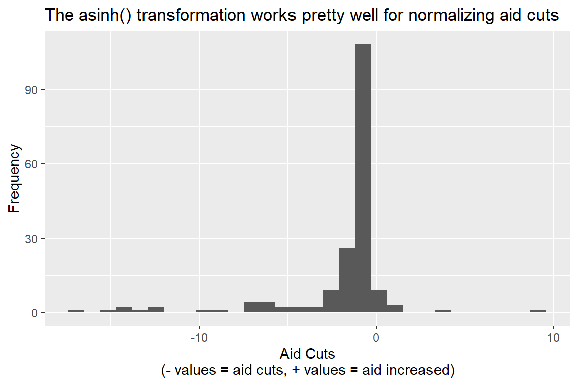
Just to cover my bases, I should check how different the distribution looks by taking the raw difference, which I do below. As you can see, this alternative way of measuring aid cuts gives me a really skewed distribution, which could create some problems when I analyze the data.
ggplot(dt) +
  aes(x = disbursed_2025 - disbursed_2024) +
  geom_histogram() +
  labs(
    title = "The raw difference looks pretty skewed"
  )
`stat_bin()` using `bins = 30`. Pick better value `binwidth`.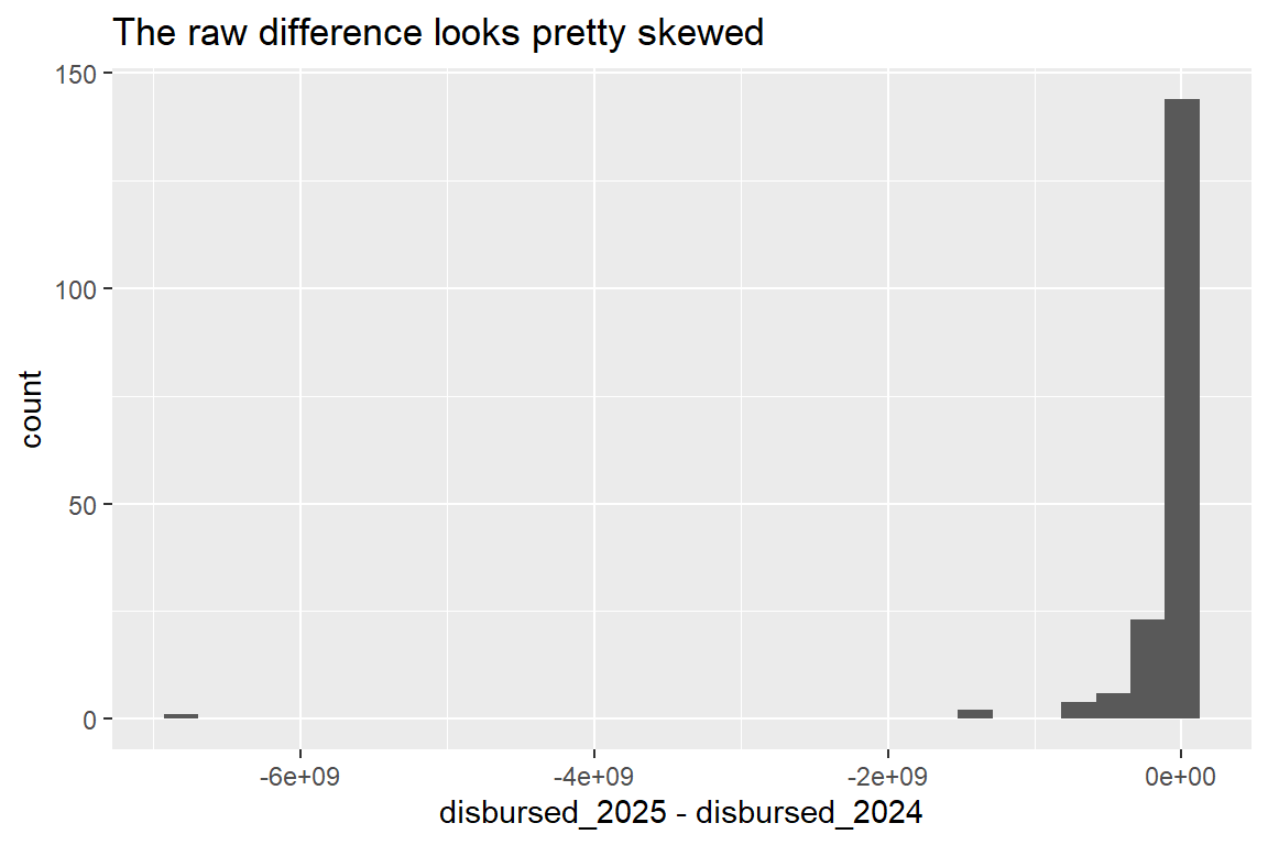
With an outcome variable defined, the next step is to think about factors in the data that might explain its variation. Let’s start simple. How about we just look at democracy scores?
This seems like a good place to start to me because, historically, one of America’s foreign policy goals was democracy promotion throughout the world. In practice, this has meant the U.S. often showed favoritism toward democratic regimes when giving foreign aid. It might be worth checking whether democracies got any kind of reprieve from U.S. aid cuts in 2025.
Before we estimate a regression model to test whether this was the case, however, we should look at the relationship with our own eyes. A scatter plot would be a good choice, perhaps with a smoothed line of best fit running through the data. I made one using the below code. Unfortunately, there are 16 observations in the data that don’t have a valid democracy score, so we lost some data points. And notice that the ones we lost were those with some of the more extreme positive aid cut values (countries that actually got more aid in 2025 than 2024). Nonetheless, among the remaining data points, there’s a noisy but discernible pattern in the data: more democratic aid recipients tend to see steeper aid cuts than non-democracies. That’s not what I expected to see.
dt |>
  drop_na(vdem_score) |> ## drop rows with missing democracy scores
  ggplot() +
  aes(vdem_score, aid_cut) +
  geom_point() +
  geom_smooth(
    method = "gam"
  ) +
  labs(
    title = "The U.S. cut more aid in democracies than non-democracies",
    x = "V-Dem Score",
    y = "Aid Cuts"
  )
`geom_smooth()` using formula = 'y ~ s(x, bs = "cs")'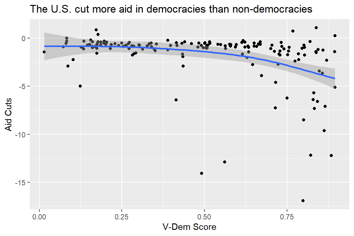
4.5.2 Estimating a simple regression model
Now that we’ve looked at the data, I feel somewhat confident that a linear model will do a fair job summarizing the relationship between democracy and aid cuts. When doing a regression analysis, it’s always a good idea (and often expected) to write out the regression model you want to estimate. This is an important step, because it makes your analysis more transparent and, thus, easier for someone else to replicate. In this case, the model can be written out like so:
\[ \text{cut}_{i} = \beta_0 + \beta_1 \text{dem}_i + \epsilon_i \]
Estimating this regression model will let us quantify how much aid cuts increase or decrease on average as democracy scores go up.
The code we need to write in R to estimate this model looks like this:
lm_fit <- lm(aid_cut ~ vdem_score, data = dt)The syntax for lm() is simple. First, provide it with a formula object. You make one by writing script that looks generically like outcome ~ explanatory_variable. In this case, I wrote aid_cut ~ vdem_score, which can literally be translated as “aid cuts, modeled as a function of democracy scores.” Next, you tell lm() the dataset it needs to look in to find the variables in the formula object. I told it to look in dt. So that I can save the results for later use, I assigned the output from the linear model function to an object named lm_fit.
Once the above code is run, the estimated model now exists in R’s memory as an object called lm_fit. Let’s call the object and see what’s inside:
lm_fit
Call:
lm(formula = aid_cut ~ vdem_score, data = dt)

Coefficients:
(Intercept)   vdem_score
    0.09278     -3.88989
Let me break down what the above output is telling you. The stuff under Call: is just meant to be a reminder of the original instructions you gave lm(): both the formula object and the data you gave it. The real action is under Coefficients:. This part tells you what the estimated model intercept and slope are. Remember that the intercept is an estimate of the mean of the outcome variable when the explanatory variable is zero, and the slope is an estimate of the change in the outcome’s average for each unit increase in the explanatory variable.
If you want to just extract the coefficients without all the extra fluff, you can use the coef() function like so:
coef(lm_fit)(Intercept) vdem_score
0.0927817 -3.8898896 Let’s take a look at the actual coefficient values and see if we can make sense of them.
First of all, the intercept is positive. This tells us that among countries that are the most autocratic (a democracy score of zero), the U.S. on average increased how much aid it gave in 2025 compared to 2024.
Second, the coefficient for vdem_score is negative, which tells us that countries with better democracy scores tended to see bigger aid cuts in 2025 on average. Because of the way the outcome was constructed, the interpretation of the magnitude of the democracy coefficient isn’t as intuitive as I would like. Remember, data transformations have consequences, and this is one of my least favorite consequences of using the asinh transformation. The technical way to interpret the coefficient is that full democracies on average got about 3.89 less asinh-transformed dollars of aid in 2025 compared to asinh-transformed dollars of aid in 2024.
I know. That’s not very intuitive. And worse yet, you have to figure out how to explain what that means to other people. Yikes!
All hope isn’t lost, however. Like I mentioned before, one bright spot with the asinh() function is that it’s approximate to the natural log. And here’s a coold feature of logs: a difference in logs is quite close to the difference in proportions. If you multiply proportions by 100, you get percentages. And people really like percentages.
Since the asinh() function is approximate to the log in scale, that means a difference in asinh-transformed variables is approximately the same as a difference in log-transformed variables and, hence, the proportion change. So, if you multiply the -3.89 coefficient estimated for democracy score by 100, it tells you that going from being a strong autocracy to a strong democracy decreases the percentage change in aid in 2025 compared to 2024 by 389 percentage points! In short, democracies lost an awful lot of aid in 2025 compared to non-democracies.
4.5.3 Estimating a multiple regression model
One of the main goals of descriptive analysis is quantifying the relationships between variables. The above analysis shows that this process is quite simple. However, in the previous example I estimated a bare-bones regression model that let me summarize how a single variable explained variation in another. This can be useful, but often times you’ll want to know how many different factors in combination explain variation in an outcome. That is, you’ll want to estimate a multiple regression model; not just a simple one.
So I propose we extend the regression analysis we did above by including some additional factors in the model. One important one we might want to consider is the level of economic development of different countries. One of the many goals behind giving foreign aid is to help developing countries, well, develop. Naturally, you’d expect donor countries to target more aid in countries that have the farthest to go in terms of economic development.
We can test for this a couple different ways. We can use the income group categories as explanatory variables in the model, or we can use gross domestic product (GDP) per capita. The latter is a standard variable in regression models of aid allocation, so let’s use it.
First, we need to add this variable to our data. We have all we need to construct it. The below code will do all the work. It creates a new column called gdp_pc which is the asinh-transformed values of 2024 GDP to 2024 population (I want to use 2024 values because it’s possible 2025 values could be affected by 2025 aid cuts—a problem known as endogeneity, which we’ll talk about later when we discuss causation). I’m using the asinh() function to normalize GDP per capita (which tends to be skewed) and because I like to be consistent about the transformations I use with data. I could use the log(), which won’t break down with GDP per capita since values are all positive, but since I used asinh() for the outcome, I feel more comfortable using it with explanatory variables, too.
dt |>
  mutate(
    gdp_pc = asinh(gdp_2024 / pop_2024)
  ) -> dt
Another factor I may want to consider is military alliances. For strategic reasons, the U.S. may want to avoid ticking off its allies, so perhaps it made shallower aid cuts to these countries. It’s a hypothesis worth testing.
I could keep adding variables, but let’s stick with three for now. Here’s the regression model I plan to estimate:
\[ \text{cut}_i = \beta_0 + \beta_1 \text{dem}_i + \beta_2 \text{GDPpc}_i + \beta_3 \text{ally}_i + \epsilon_i \]
And here’s the R code that will estimate this model for me:
multi_fit <- lm(aid_cut ~ vdem_score + gdp_pc + any_alliance, data = dt)Let’s take a look at the results:
coef(multi_fit) (Intercept) vdem_score gdp_pc any_alliance
4.2103014 -3.3663909 -0.4725581 0.6420599 Okay, these estimates look interesting. But first let me flag something really important. Multiple regression uses all the explanatory variables in the model to adjust for how each individual explanatory variable explains variation in the outcome. Notice, for example, that the coefficient for democracy score is slightly different compared to its estimate in the simple regression model. It’s -3.36 instead of -3.89.
The reason the estimate is different is that GDP per capita and alliances are “absorbing” some variation in aid cuts not explained by democracy, and they’re doing the same for democracy itself.
A good explanation for why this happens comes in the form of the Frisch-Waugh-Lovell Theorem. You should read more about it if you have time, but the gist of it is simple.
In the case of the model explaining variation in aid cuts, imagine that under the hood there are a succession of regression models taking place. One uses GDP per capita and alliances to explain democracy, and the other uses GDP per capita and alliances to explain aid cuts. Those models can’t explain all the variation in democracy and aid cuts, which gives you left-over variation in each. That left-over variation is then what gets used to estimate the relationship between democracy and aid cuts. Something similar happens for GDP per capita and alliances, too.
All this means, by the way, that you should be careful about what factors you throw into a multiple regression model. Remember that regression models rely on two key assumptions: (1) that you’re data is valid and (2) that the outcome can be modeled as an additive function of separate covariates. In a multiple regression model, because it’s as though you’re working with many nested layers of regression models, these assumptions have to be met for each nested layer. The more variables you add to your model, the more these assumptions multiply and the greater the risk that they’re violated.
This problem is so pernicious that one famous political scientist made the rather controversial argument that no one should estimate a regression model with more than three explanatory variables. His name is Christopher Achen, and his argument is called “a rule of three” (or ART for short). He claimed that beyond three explanatory variables, it becomes exponentially hard to empirically verify if a regression model’s key assumptions are being met. Therefore, he says you should be suspicious of regression results based on models with four or more explanatory variables.
That’s a tall order, and in practice few political scientists follow this advice. In fact, most of us think derisively about it. But if you take ART less literally, but still seriously, the point that you should be careful about what variables you put in a regression model is well taken. Statistical software makes it trivially easy to add dozens (even hundreds) of variables to a regression model. Doing so without first thinking carefully about the factors going into a model is a bad idea. Model creation isn’t just a mechanical act of adding some variables to a formula. It’s a craft that requires thoughtfulness, attention to detail, and (dare I say) some creativity.
These are points you’d do well to remember, especially in this dawning age of AI software where it will become increasingly tempting to automate the process of data analysis. You should strive to play an active role in research. Without human creativity, attention to detail, or thoughtfulness, I can see a future world awash in garbage regression models that generate meaningless results.
Any way…back to talking about the regression results. Overall, the multiple regression model tells us that it identified some interesting patterns in the data. Let me show you those results again below:
coef(multi_fit) (Intercept) vdem_score gdp_pc any_alliance
4.2103014 -3.3663909 -0.4725581 0.6420599 The model tells us that the U.S. cut more aid in democracies than non-democracies, and in countries with higher levels of economic development (the coefficient for GDP per capita is negative). Conversely, the U.S. didn’t cut as much aid to its allies (the coefficient is positive). These are interesting results. It seems that the U.S. may have been somewhat strategic with its aid cuts in 2025.
Maybe. But before we can draw this conclusion we need to quantify the role that chance played in giving us these regression estimates. This is the subject of the next chapter. Quantifying how random chance (or noise) might explain variation in data is a critical step in descriptive data analysis. While it’s helpful to be able to quantify patterns that exist in data, we also want to know whether the patterns we observe had a high or low chance of happening as a result of pure dumb luck. This is the role that statistics plays in data analysis, and it adds an extra layer of rigor to descriptive research. It raises the bar required to claim that some result isn’t the product of random chance. Until we take this step, we don’t know if the variation in aid cuts explained by democracy, GDP per capita, or alliances is statistically significant (a term used to signal that a result had a very low chance of happening due to dumb luck). So let’s raise the bar in the next chapter and see what we find.
4.6 Wrapping up
I know that there’s a lot to absorb in this chapter. On the theoretical side, I talked about data models in the abstract and how to use objective functions and estimators to fit them to data. I also talked about some of the basic building blocks of linear models and how to fit these models using OLS. Finally, I did some applied examples using R to fit regression models of U.S. aid cuts.
I don’t expect you to master all these details in one reading. Instead, my goal was to create a resource for you to come back to if you ever get lost. Also, it may encourage you to know that linear regression is the exclusive model we’ll be using in all subsequent chapters. So while the material here is dense, it applies across almost everything else we’ll do in the rest of the course.
There are, however, many models other than linear regression. Linear models aren’t inherently better than these alternatives. That’s not why I’ve chosen to focus only on linear regression. I’ve made this choice because I think it’s better for your own educational journey to understand one kind of model with some level of confidence rather than to expose you to many models that you don’t have time to understand. I never learned very well through broad, surface level exposure, and I’m going to assume that you don’t learn very well through this approach either. I need to spend some time with a single topic before I’m ready to go further, and I’m making the assumption that you need to spend some time with a single topic for a bit, too.
Another reason to focus on linear models is that many other common models were created by people who were familiar with linear regression but needed to solve a specific problem with how linear regression performed in a certain setting. In one way or another, the linear model is the the inspiration for a wide range of alternative models. So if you can wrap your head around linear regression, I think you’ll have an easier time understanding more sophisticated models down the road.
Coming up, now that we’ve covered linear models, in the next chapter we’re going to talk about statistical inference. This is the process of quantifying the role of chance in explaining trends or relationships in data. As we’ll discuss, quantifying trends in data is great, but statistical inference adds a layer of rigor by forcing us to evaluate whether the patterns we see in data really are patterns or just random noise.