7 Model Validation and Selection
7.1 Goals
Learning objectives:
- The goal of predictive modeling is to make good predictions.
- There are many methods that we can use to determine if a model is reasonably good, and to compare different competing models to identify the best.
- We’ll talk about one method called leave one out cross-validation that is useful for making a predictive model of U.S. presidential elections.
7.2 Assessing predictive accuracy
The goal with predictive analysis is to develop a good forecast model for whatever outcome is of interest. Researchers use predictive models to predict what consumers will buy, what the weather will be tomorrow, and how people will vote in elections. In some cases, getting predictions wrong isn’t just annoying, it can be costly. Companies want to maximize their profits by knowing how to target adds at consumers, public officials want to know whether they need to tell citizens to evacuate before a hurricane makes landfall, and political campaigns want to know how best to invest their resources to improve their chances of taking or holding onto office.
So how do you know if you have a good predictive model? In the context of elections, this is a really hard question to answer because elections don’t happen every day. It’s far easier to predict consumer behavior and the weather (yes, even the weather!). People buy things all the time, and the weather never stops. Elections, particularly in the U.S., only happen at discrete intervals years apart. In the case of U.S. presidential elections, this is every four years. There aren’t many opportunities to refine a predictive model on the fly. You only get one chance every four years to get your forecast right. That’s a lot of pressure.
The infrequency of presidential elections makes verifying the predictive accuracy of forecast models difficult for the simple reason that verifying whether your model is good requires making predictions with new data. If you only get new data every four years, it takes a long time to validate your model.
However, don’t lose hope. While the true test of a model is its accuracy when you take it out into the real world, there are methods that allow you to take your model for a test drive before you make a down payment and drive it off the dealer’s lot for good. I want to introduce you to some of these methods in this chapter, and walk you through some R code that allows you to implement these methods using the presidential election data I introduced in the last chapter.
7.3 Background on cross-validation for checking model performance
Cross-validation is an approach to testing model performance that is, to keep using the car dealership analogy, a lot like taking a car you’re interested in buying for a test drive. It gives you an opportunity to get a feel for how a car will perform on the road, whether it’s a comfortable ride, and whether it seems safe and in good condition. There are no guarantees, however. Everything could seem just fine on the test drive while later on you discover you were sold a lemon. Nonetheless, your chances of making a good purchase are far higher if you take the time to test drive a car, or ideally several, before you make a final decision.
I could belabor this analogy a lot more, but I hope you get the intuition. Cross-validation offers a way to get a sense for how a model might perform when confronted with new data.
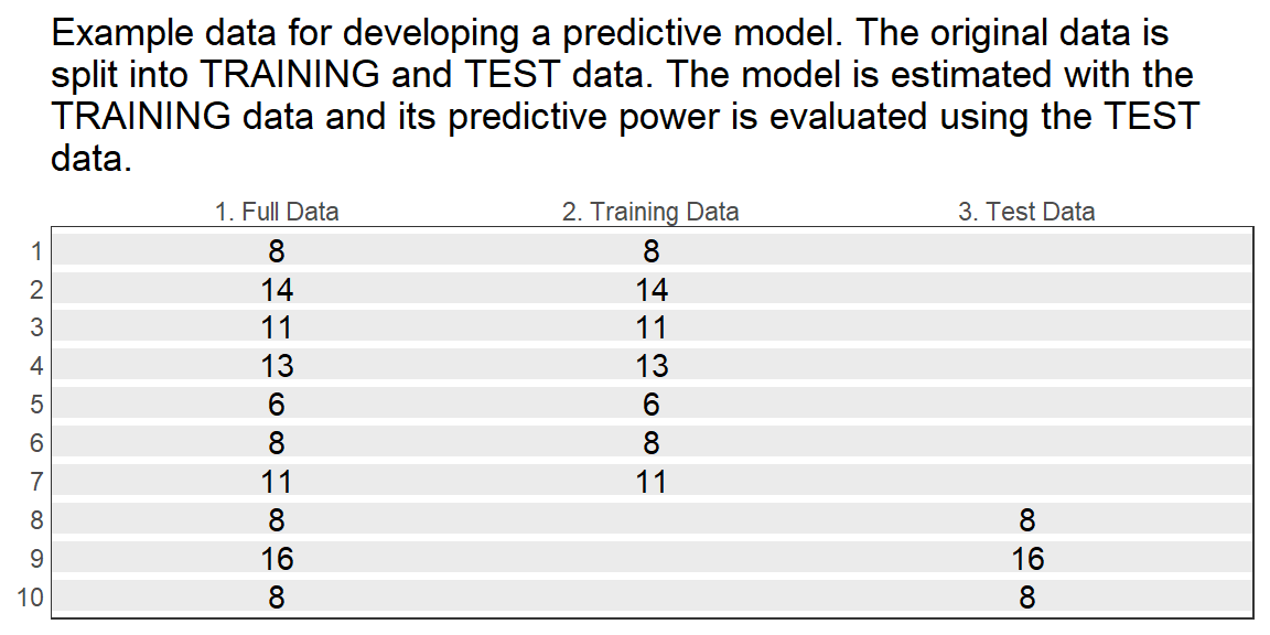
What exactly is cross-validation? It isn’t just one thing; it comes in a few different varieties. But all of these variations share one thing in common. Cross-validation is all about fitting your predictive model to some of your data, and then using the rest to validate how well your model performs. The below figure visualizes what this means. You start with your full dataset. You then split it into a training set and a test set. You use the training data to estimate your model, then you use the test data to check the quality of your model’s predictions. There are no hard and fast rules for how large the training data should be relative to the test data, but a common practice is to retain at least 70% of the data in the training set.
It’s possible to perform this split just once, but cross-validation methods involve repeating this process of leaving some data out, fitting the model, and predicting the leftovers multiple times. There are several versions of what this can look like, but there are three basic flavors I want to introduce you to that I think offer a general sense for what cross-validation can entail.
Here are the main three I want to talk about:
- Monte Carlo Cross-validation (MC)
- k-fold Cross-validation (k-fold)
- Leave-one-out Cross-validation (LOO)
Monte Carlo Cross-validation (let’s just call it MC) involves splitting the data at random and validating a model an indefinite number of times. I sometimes liken this approach to bootstrapping minus replacement. The idea is you pull out a random subset of your data, fit your model with it, then predict the leftover subset. You repeat this process a bunch of times and what you end up with is a range of values indicating how well your model performed on the various test datasets.
k-fold Cross-validation (just k-fold for short) is a more organized cousin of MC. Rather than sample the data at random, it calls for lumping the data into a discrete number of buckets that will be pulled out one at a time as test data sets. How many buckets? The letter “k” is a stand in for however many buckets you choose. Obviously, the larger your data, the higher the number of buckets can be, however 5-fold and 10-fold varieties are quite common. The main difference between this approach and MC is that the k-fold buckets are fixed. That means if an observation is pulled out for the test data in round 1 of the k-fold procedure, it can never be pulled out again in subsequent rounds. With MC, any observation is fair game across all the iterations you might choose to run.
Leave-one-out Cross-validation (LOO) is k-fold taken to its extreme. As the name implies, you leave out one observation from the data at a time and use the rest of the data to see how well you can predict the one that was left out. This kind of approach is sometimes called a jackknife. Like with k-fold, once an observation has been pulled out, it can never be pulled out again.
There are bias-variance trade offs associated with these alternative cross-validation methods. I talked about this problem a few chapters ago when I discussed statistical uncertainty. It’s possible to have an estimate that is likely to be close to the truth on average but that is subject to lots of noise. It’s also possible to have an estimate that tends to run afoul of the truth on average but that is subject to very little noise.
MC tends to have low variance, but high bias. k-fold, on the other hand, has low bias, but high variance. LOO actually tends to be good with respect to both bias and variance, but this comes at the cost of computational efficiency. If you have a very large dataset, LOO can take forever to run. But, if you have a relatively small data sample it’s a really good choice. For predicting presidential elections, LOO therefore has a lot of advantages as a cross-validation strategy because the universe of elections we have to work with is fairly small, so compute isn’t a limiting factor.
7.4 Measuring and comparing model performance using RMSE
Once you have a cross-validation strategy, you need to decide how you will measure predictive performance. There are many such measures, but I want to introduce you to one of my favorites. It’s called root mean squared error or just RMSE. It’s my preferred metric because it has an intuitive interpretation. RMSE tells you how much, on average, your prediction differs from the truth. That means the bigger the RMSE, the bigger the errors your model makes on average.
It’s quite easy to calculate. Say you have the following regression model:
\(y_i = \beta_0 + \beta_1 x_i + \beta_2 z_i + \epsilon_i\)
After you fit it to your training data, you generate a set of predictions \(\hat y_i\) for all the observations you included in your test data. To calculate the RMSE for your predictions, you just need to use the following equation:
\(\text{RMSE} = \sqrt{\frac{\sum_i(y_i - \hat y_i)^2}{N}}\)
In the above, \(N\) is the number of observations in your test set.
The value in having a metric like RMSE is that you now have a way to benchmark how well your model performs. It also gives you a basis for validating many competing models and identifying the one that yields the best accuracy. This is called model selection.
When using RMSE, you would select a model on the basis of which one gives you the lowest RMSE. In short, you would select the model that makes the smallest errors on average.
7.5 Cross-validation and model section in R
The R programming language comes with some helpful tools for doing cross-validation. I’ll show you a package called {modelr}, which provides tools that mesh well with the {tidyverse} that are specialized for working with models.
If you don’t have the package, you first need to make sure you get it installed by running the following code in your R console:
install.packages("modelr")Let’s read in the presidential election data we used in the last chapter, and then walk through some examples for how to do cross-validation.
## packages we need
library(tidyverse)
library(estimatr)
library(modelr)

## function to simulate predictions with uncertainty
sim_pred <- function(model, newdata, its = 1000) {
  if(missing(newdata)) stop("The 'newdata' option is missing.")
  if(!identical(class(model), "lm_robust")) stop("The model should be a 'lm_robust' class object.")
  sim_pres <- replicate(
    n = its,
    expr = {
      nmodel <- model
      nmodel$coefficients <- MASS::mvrnorm(
        n = length(model$coefficients),
        mu = model$coefficients,
        Sigma = nmodel$vcov
      ) |> diag()
      ndata  <- newdata
      ndata$pred <- predict(nmodel, newdata = newdata)
      list(ndata)
    }
  )
  out <- dplyr::bind_rows(sim_pres)

  ## return out
  out
}

## read in the data
presdt <- read_csv(
  "https://tinyurl.com/pres-forecast"
)
I introduced this data in the last chapter. As quick refersher, the data has information related to all presidential elections that have taken place from 1948 to 2020. The 2024 election has already happened, but say it hadn’t and we wanted to develop the best forecast model we could for the election. Our workflow would be straightforward:
- Come up with a short-list of predictive models.
- Use cross-validation and RMSE to identify the best one.
- Make some predictions using the model we selected.
Let’s tackle these steps one at a time.
7.5.1 Models to compare
One compelling model of presidential elections is called the political economy (PE) model, which has been in use for a long time. It has a generally good track record and a very simple formulation. The PE model specifies that the incumbent party’s presidential vote margin is a function of two things: (1) economic growth and (2) the incumbent party’s approval rating.
There are variables that capture each in the data, so this model is no-brainer to consider. But there are other factors in the data to look at, too. Inflation might also be important, along with the presence of a third party challenger. I’ll make another model called PE-plus that adds these factors to the classic PE model.
I’m sure we could come up with more, but I’ll stick with two models for this example to keep things simple.
First, I need to encode these models in a convenient way for doing cross-validation. Here’s one strategy to consider. In the below code rather than fit models to the data right off the bat, I’m going to create a list containing the model formulas I want to use. This is a convenient way to save this information for later use in the cross-validation step.
forms <- list(
    inc_vote_margin ~
      gdp_pct_change + inc_net_approval,
    inc_vote_margin ~
      gdp_pct_change + inc_net_approval +
      third_party_present + inflation_pct_change
  )
7.5.2 LOO for model selection
As I mentioned before, the LOO method for cross-validation is a great choice for relatively small datasets. There are just 19 observations in the presidential election data, so I think this qualifies as a small dataset.
The {modelr} package has specific cross-validation functions that will generate the cross-validation training and test sets I need to perform the procedure. There’s a distinct function for each of the three methods I introduced earlier: crossv_mc() for MC, crossv_kfold() for k-fold, and crossv_loo() for LOO. Since I’m going with LOO, I’ll use the last one.
This function is really simple to use. By just writing the following code, the function will generate an object that contains every possible training and test dataset I could get with the presidential election data using LOO. In this case, there are 19 versions of each. I made sure to save this object as cvdt.
cvdt <- crossv_loo(presdt)Take a look at the first five rows of this object. As you can see, it contains some very special values. There’s a column called train, one called test, and one called .id. The first is the set of all training datasets I get by dropping one observation at a time. The second is the set of all left-out rows of the dataset. The last is just an identifier for the cross-validation sets. There are 19 since there are 19 rows in the data to leave out.
cvdt |>
  slice_head(n = 5)
# A tibble: 5 × 3
train test .id
<named list> <named list> <int>
1 <resample [18 x 12]> <resample [1 x 12]> 1
2 <resample [18 x 12]> <resample [1 x 12]> 2
3 <resample [18 x 12]> <resample [1 x 12]> 3
4 <resample [18 x 12]> <resample [1 x 12]> 4
5 <resample [18 x 12]> <resample [1 x 12]> 5Now that I have the cross-validation sets, I need to fit my models to the training datasets and then calculate the RMSE using the left out observations.
The first step is to incorporate the model formulas I created earlier into the LOO data object. To do this, I need to solve a problem. There are multiple versions of the model that I want to try per cross-validation set, but the cvdt object has just one row per set. In the below code, I use the function expand_grid() to solve this problem. I first tell it that I want a column called forms equal to the forms object I created earlier. I then also give it the cvdt object I created above. I assign the output from this function to cvdt giving me a new version of this object that has been modified.
cvdt <- expand_grid(
  forms = forms,
  cvdt
)
Take a look at this object now. The below code shows the first five rows. Everything looks the same, except there is now a forms column.
cvdt |>
  slice_head(n = 5)
# A tibble: 5 × 4
forms train test .id
<list> <named list> <named list> <int>
1 <formula> <resample [18 x 12]> <resample [1 x 12]> 1
2 <formula> <resample [18 x 12]> <resample [1 x 12]> 2
3 <formula> <resample [18 x 12]> <resample [1 x 12]> 3
4 <formula> <resample [18 x 12]> <resample [1 x 12]> 4
5 <formula> <resample [18 x 12]> <resample [1 x 12]> 5This isn’t all. If I use the dim() function R will tell me how big this object is in terms of rows and columns. Check it out: I now have double the number of rows as before (38 compared to 19). This because the cross-validation sets now repeat so that each one is matched to each of the model specifications I want to test.
dim(cvdt)[1] 38 4The next step is to fit the models to the training data. The below code is a little more involved for model fitting than what you’ve seen so far. The reason is that I want to save the model fits as a column in this cvdt object. The below code uses the mutate() function to let me add a new column to the data that I want to call fit. To make this column I’m using a function called map2() which comes from the {purrr} package (part of the {tidyverse}). This function lets me repeatedly apply a function based on two inputs in each row of the data, represented by the .x and .y options. I’ve told map2() that .x will represent values in the forms column and that .y will represent values in the train column. map2() then lets me specify the function/operation that I want to give these inputs to. In this case, I’ve told it that I want to give them to lm() where .x will be the model formula and .y will be the data. This little bit of code lets me automate the process of estimating 38 regression models all without having to actually write out the code line by line to do so.
cvdt <- cvdt |>
  mutate(
    fit = map2(
      .x = forms,
      .y = train,
      .f = ~ lm(.x, data = .y)
    )
  )
Once I have the model fits, I then have to calculate the RMSE. Thankfully, {modelr} has a function called rmse()that I can apply to each of my models to calculate this quantity. It expects two potential inputs: a model and data. If you don’t supply data, it will give you the RMSE using the original data used to estimate the model. If you give it data, it will base the calculation on the observations in it instead. Like in the previous code, I need to use map2() since I need to apply rmse() to each unique model and test data set.
cvdt <- cvdt |>
  mutate(
    rmse = map2(
      .x = fit,
      .y = test,
      .f = ~ rmse(model = .x, data = .y)
    )
  )
If you look at the output, you’ll notice that rmse is in an unusual format. Rather than just indicating the RMSE, the data is saved as a list. I can fix that using the unnest() function:
cvdt <- cvdt |>
  unnest(rmse)

cvdt |>
  slice_head(n = 5)
# A tibble: 5 × 6
forms train test .id fit rmse
<list> <named list> <named list> <int> <list> <dbl>
1 <formula> <resample [18 x 12]> <resample [1 x 12]> 1 <lm> 0.0251
2 <formula> <resample [18 x 12]> <resample [1 x 12]> 2 <lm> 0.0411
3 <formula> <resample [18 x 12]> <resample [1 x 12]> 3 <lm> 0.00725
4 <formula> <resample [18 x 12]> <resample [1 x 12]> 4 <lm> 0.0547
5 <formula> <resample [18 x 12]> <resample [1 x 12]> 5 <lm> 0.00860I now have a distribution of RMSE values for each version of the model. Now I can begin the process of comparing them and selecting the best one. But first, I need to include a column that categorizes the models by which one they are: either PE or PE-plus. The first 19 are the PE specification and the second 19 are PE-plus. The below code applies the correct labels for each and saves them in a new column called model.
cvdt <- cvdt |>
  mutate(
    model = rep(
      c("PE", "PE-plus"),
      each = 19
    )
  )
Now I can visualize and compare the results. Amazingly, it looks like the simpler PE model outperforms the more complex PE-plus model. The difference is quite small, but it is there. To show this, in the below figure I lined up the data on the x-axis by the LOO iteration. On the y-axis I showed the RMSE associated with each iteration, and I mapped the color aesthetic to whether the model in question is PE or PE-plus. I used geom_point() to represent each model specific RMSE as dots, and then I used some tricks with geom_smooth() to get it to return just a horizontal line indicating the overall average RMSE for each model.
ggplot(cvdt) +
  aes(x = .id, y = rmse, color = model) +
  geom_point() +
  geom_smooth(
    method = "lm",
    se = F,
    formula = y ~ 1
  ) +
  labs(
    x = "LOO iteration",
    y = "RMSE",
    color = "Model",
    title = "PE performs a hair better than PE-plus",
    subtitle = "Dots are the iteration specific RMSE and the horizontal lines\nare the overall average RMSE"
  )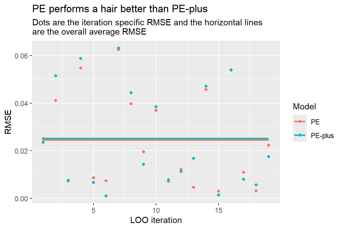
Based on these results, I’d probably stick with the PE model. The difference in RMSE on average isn’t practically substantial, which means PE-plus, despite bringing in additional information, isn’t improving accuracy. If two or more models perform about the same, a good rule of thumb is to select the simplest among your options.
7.5.3 Make predictions
Once you have a model selected, you can then generate some predictions. Importantly, when you shift from validation to prediction, I would recommend including all the data back into your model estimation. You’ve already taken the model for a test run, now gun it and see what happens.
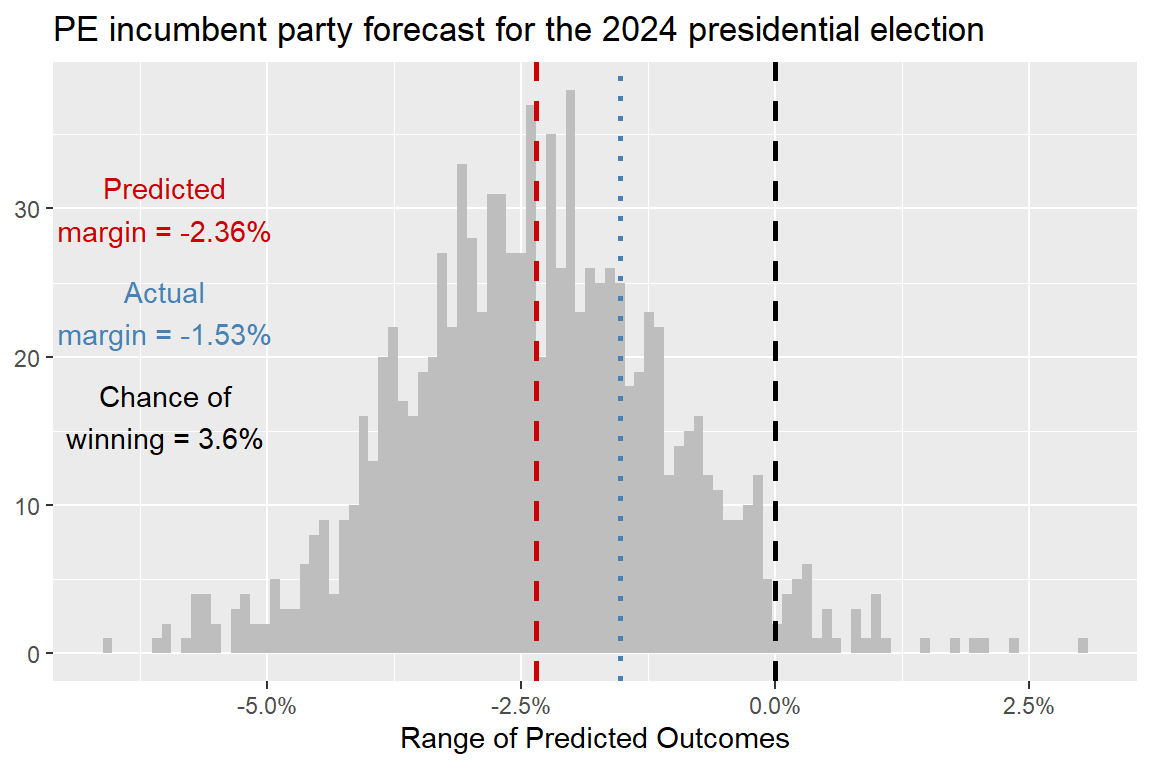
In the below code I fit the PE model to the full dataset from 1948-2020. I then use sim_pred() to generate a range of predictions for the 2024 election that the model is consistent with. I gave the function updated values for 2024 for the predictor variables in the model. For GDP growth (gdp_pct_change) I just looked up what U.S. GDP growth was in 2024, and I did the same for incumbent party net approval (specifically approval as of June 2024). I then had sim_pred() simulate outcomes for the 2024 election, which I then gave to ggplot() to visualize. I could have made any number of predictions, but in the below I decided to use a histogram summarizing the distribution of simulated predictions with vertical lines and labels indicating what the average prediction was and the threshold needed to secure a majority of the vote. Since I have simulated values, I am also able to calculate the percentage of predicted outcomes consistent with incumbent victory. The PE model forecast doesn’t look so good for the 2024 incumbent party. Also, the model did pretty well. I included the actual two-party vote margin in the plot, too. The final result is well within the range of predicted values consistent with the model.
## Estimate the model using the full dataset
pem <- lm_robust(
  inc_vote_margin ~
    gdp_pct_change + inc_net_approval,
  data = presdt,
  se_type = "HC1"
)

## Simulate predictions
pem_forecast <- sim_pred(
  pem,
  newdata = tibble(
    gdp_pct_change = 2.8,
    inc_net_approval = -20
  )
)

## Actual margin in 2024
dem <- .483
rep <- .498
mar <- (dem - rep) / (dem + rep)

## Visualize the results
ggplot(pem_forecast) +
  aes(pred) +
  geom_histogram(
    bins = 100,
    fill = "gray"
  ) +
  geom_vline(
    aes(
      xintercept = mean(pred)
    ),
    linetype = 2,
    color = "red3",
    linewidth = 1
  ) +
  geom_vline(
    aes(xintercept = mar),
    linetype = 3,
    color = "steelblue",
    linewidth = 1
  ) +
  geom_vline(
    xintercept = 0,
    linetype = 2,
    color = "black",
    linewidth = 1
  ) +
  annotate(
    "text",
    x = -.06,
    y = 30,
    label = paste0(
      "Predicted\nmargin = ",
      mean(100 * pem_forecast$pred) |>
        round(2), "%"
    ),
    color = "red3"
  ) +
  annotate(
    "text",
    x = -.06,
    y = 23,
    label = paste0(
      "Actual\nmargin = ",
      mean(100 * mar) |>
        round(2), "%"
    ),
    color = "steelblue"
  ) +
  annotate(
    "text",
    x = -.06,
    y = 16,
    label = paste0(
      "Chance of\nwinning = ",
      mean(100 * (pem_forecast$pred > 0)) |>
        round(2), "%"
    )
  ) +
  scale_x_continuous(
    labels = scales::percent
  ) +
  labs(
    x = "Range of Predicted Outcomes",
    y = NULL,
    title = "PE incumbent party forecast for the 2024 presidential election"
  )
7.6 Summary
Cross-validation is an important step in developing any predictive model. While it offers no guarantees, it’s the best approach for assessing how good a model can be expected to perform when confronted with new data.
I want to wrap up with a quick note about other methods of model selection, and a warning about using them. One common approach that somehow keeps showing up in classroom settings, despite its well known flaws, is stepwise regression. Like cross-validation, this approach involves an iterative process of re-estimating models. Unlike cross-validation, stepwise regression doesn’t involve making predictions with new data. Instead, you use metrics of within-sample performance, like the R-squared value, to judge performance. As a result, this approach sensitive to statistical noise and may give you a bad recommendation for a predictive model.
A less systematic approach than stepwise regression that is equally problematic is to simply estimate a series of models and then reject ones that have statistically insignificant predictors. The reason, again, is that the statistical significance of these predictors tells you nothing about how well they predict new outcomes.
These approaches, and any others that use within-sample predictions to validate and select models risk the problem of overfitting. I talked about this in the last chapter. Overfit models are those that are so finely tuned to predicting an outcome using a particular dataset that they struggle to generalize to new observations. By using out-of-sample predictions, cross-validation lets you simulate how well your model does when confronted with new data, thus helping you to avoid making a model that’s too specialized.
Cross-validation can’t guarantee that your model is perfect. This point is worth making clear. However, it does offer you a well-founded and evidence-based way to make an informed judgement. Often, this is the best you can hope for when working with real-world data.