library(tidyverse)
url <- "https://raw.githubusercontent.com/milesdwilliams15/Teaching/main/DPR%20201/Data/aidExperiment.csv"
Data <- read_csv(url)9 Randomized Controlled Trials
9.1 Goals
Learning objectives:
- Randomized experiments provide the best way to make causal inferences.
- The randomization process helps avoid the problem of bias or confounding in data.
- There are lots of tools in R for doing randomization and estimating treatment effects.
- There are many kinds of estimators of treatment effects, including the average treatment effect (ATE), the intent to treat effect (ITT), and the compliers average treatment affect (CATE).
9.2 Introduction
A randomized controlled trial (RCT) is a research design that lets you get an unbiased estimate of an average treatment effect (ATE). By randomly assigning a policy intervention (treatment), it ensures other confounding factors don’t bias the results.
Think of it this way. The world is a complicated place, with lots of known and unknown factors that can bring about different relationships between factors in the world. Take the correlation between a country being a major oil exporter and whether it is a democracy. If you tabulate the data, you would see that countries where oil is more than 50% of their exports also tend to be autocratic (the opposite of a democracy).
But how do you know whether this relationship is causal? If you could flip a switch and make the oil stop flowing in these countries, do you think you could turn them into democracies? Maybe. But there could be other, deep historical reasons why these countries remain autocratic as well, and these factors could also be correlated with geography and natural resources, such as oil. So it’s hard to say that this one change is sufficient to bring about democracy.
Questions like this are hard to find good answers to, but they are important to ask. In the world of politics and policy, before you think about how you would want to intervene in the world to make it a better place, you need to think seriously about how confident you are that X intervention will lead to Y outcome. Shutting off the flow of oil in an autocratic country is probably beyond your reach, but there are many hypothetical and realistic policy interventions that are nearer to home. Will body cams lead to better policing? Will increasing the minimum wage come at the cost of lower employment? Are progressive tax systems a reliable means of supporting public services that benefit the lower and middle classes? Could a proportional voting system better the chances of third parties in US politics?
Not all of these questions can be realistically answered using randomized experiments, but using the logic of a randomized experiment can help discipline your thinking. What kind of evidence would you need to feel confident that a proposed policy intervention or change will have the desired outcome? If you propose a policy, even a pie-in-the-sky policy, you need to ground your recommendation in evidence. Randomized controlled trials are the first kind of research design you should consider.
I talked a little bit about how randomization is important for making causal inferences in the last chapter. However, there are many different ways to go about randomization. While RCTs are a unique kind of research design, there is lot of diversity among RCTs in terms of how units are assigned to treatment or control. In the next section, I’ll use the {randomizr} R package to walk through a few different techniques. These include simple randomization, complete randomization, block randomization, and cluster randomization.
It’s important know about these different methods for randomly assigning treatment for a couple of reasons. One is that they can be really useful in different contexts. As you’ll see, some kinds of policy interventions or problems aren’t amenable to run-of-the-mill randomization. Thankfully, you have options when this isn’t the case.
The second reason I need to talk about these different methods is that they influence how you analyze the results of an experiment. How your randomize determines how you analyze.
Okay, let’s get to it.
9.3 Random Treatment Assignment with {randomizr}
The {randomizr} package was created to give researchers doing field, lab, survey, or online experiments tools to automate the process of random assignment. You can read more about the package here: https://declaredesign.org/r/randomizr/.
The package provides functions that make it easy to implement randomization according to five different common research designs:
- Simple randomization
- Complete randomization
- Block randomization
- Cluster randomization
- Block-cluster randomization
To keep things simple, I’ll focus on the first four. For each I’ll consider scenarios where there are only two treatment conditions (that is, treatment or control). There are many studies that rely on multiple treatment conditions. These are called multi-arm treatments. These might look like variations of a treatment condition or versions of a treatment with a different dose. There are also factorial designs where there are multiple treatments, and it is possible for one unit to fall into more than one treatment condition at once. However, before you start thinking about these additional research designs, it’s important to master the basics. That’s the focus of this chapter.
For each of these kinds of randomization, pretend like you were able to run an experiment using some survey data. You can read into R by writing the following code:
You can run the following code to take a glimpse of what’s in the data:
glimpse(Data)Rows: 1,289
Columns: 12
$ aid <dbl> 1, 0, 1, 0, 0, 0, 1, 1, 1, 0, 0, 0, 1, 1, 1, 1, 1, 1, 1, 0…
$ gender <dbl> 0, 0, 1, 0, 0, 0, 1, 1, 1, 1, 0, 1, 0, 1, 1, 0, 1, 0, 0, 0…
$ educ <dbl> 3, 5, 3, 3, 3, 2, 3, 5, 5, 5, 5, 5, 2, 3, 6, 5, 2, 3, 6, 2…
$ relimp <dbl> 2, 4, 3, 3, 4, 2, 2, 1, 3, 1, 1, 4, 3, 3, 2, 1, 3, 1, 1, 3…
$ treat_cash <dbl> 0, 0, 0, 1, 1, 1, 1, 1, 0, 1, 1, 0, 1, 1, 1, 1, 0, 0, 1, 1…
$ treat_black <dbl> 0, 1, 1, 0, 0, 1, 1, 0, 1, 1, 0, 0, 1, 1, 1, 0, 1, 1, 1, 1…
$ loinc <dbl> 1, 0, 0, 0, 0, 0, 0, 0, 0, 0, 0, 0, 0, 0, 0, 0, 0, 0, 0, 0…
$ age <dbl> 28, 37, 68, 55, 71, 69, 73, 58, 66, 43, 42, 40, 79, 59, 61…
$ fullemploy <dbl> 1, 1, 0, 1, 0, 0, 0, 0, 0, 1, 1, 1, 1, 0, 0, 1, 0, 1, 1, 1…
$ ties3 <dbl> 0, 1, 2, 0, 0, 0, 0, 0, 1, 1, 0, 1, 1, 1, 2, 0, 0, 0, 1, 1…
$ lib <dbl> 1, 0, 0, 0, 0, 0, 0, 1, 1, 0, 0, 0, 0, 0, 1, 1, 0, 1, 1, 0…
$ race3 <dbl> 1, 1, 3, 1, 1, 1, 1, NA, 1, 1, 1, 1, 1, 3, 1, 1, 1, 1, 1, …This dataset comes from a study published in 2020 in International Studies Quarterly that looks at support for foreign aid by the American public. The aid column equals “1” if an individual supports a foreign aid project and “0” if they don’t. The other columns provide some other background information about individual respondents.
There are also two columns that refer to two different experimental conditions respondents were exposed to. One is called treat_cash and the other is called treat_black. To see if different ways of framing an aid project would influence public attitudes about cutting foreign aid, some people were given modified vignettes (these are little examples of a foreign aid project that give people some background on it) where some people were given different information at random. When treat_cash = 1, people were told that the aid program is actually domestic rather than foreign. When treat_black = 1, people were told that the aid program is in an African country rather than some generic country.
The results from this experiment are interesting, but ignore these treatments for now. Instead, pretend that you’re adding some new treatments to the data using some different RCT designs. Let’s start with a standard randomized trial.
9.3.1 Simple randomization
As the name implies, simple randomization involves just assigning each individual in the data the same probability of getting treatment and then letting a random number generator do its thing. The relevant function from the {randomizr} package is simple_ra(). Here’s some example code for how to use it:
library(randomizr)
Data |>
  mutate(
    simpleTr = simple_ra(N = n())
  ) -> Data
The thing about simple randomization is that you can end up, by random chance, with unequally sized treatment and control groups. The below code counts up the number of unique instances of the different treatment conditions you just generated. As you can see, the numbers aren’t equal.
Data |>
  count(simpleTr)
# A tibble: 2 × 2
simpleTr n
<int> <int>
1 0 648
2 1 641This isn’t always a big deal, but in many real-world scenarios you might have a fixed number of treatments you can actually assign. One good example is a study I helped with during my time at the U.S. Office of Evaluation Sciences dealing with Montana wildfires. Wildfires are a problem in Montana, in case you weren’t aware, and there are services that government agencies like USDA provide to help people “fire proof” their property. One of these services is an inspection, where someone from the forest service will come to your property and inspect it for vulnerability to forest fires. After the inspection, they’ll offer recommendations to property owners on how they can reduce their susceptibility to fire damage.
The problem is that many people don’t take advantage of this service. It isn’t mandatory. The federal government can’t force their way onto people’s properties to do this inspection. Instead, people have to submit a request. So how do you get people to actually do this?
OES decided a good tactic might be to send people letters informing them about the risks of forest fires and telling them about this available service. But, because they also wanted to build evidence that these letters could be effective, they randomly selected which property owners would be mailed a letter. Afterward, they collected data on which households requested an inspection. Turns out, the letters were effective. Those who got one were about 5-6 percentage points more likely to request an inspection (a small but statistically significant effect).
Getting back to the point about a fixed number of treatments, there were only so many letters that were budgeted for in this study. So a simple randomization wasn’t going to do. Instead, OES needed to use complete randomization, which I’ll talk about next.
9.3.2 Complete Randomization
You can use complete_ra() for complete randomization. Here’s some example code:
Data |>
  mutate(
    completeTr = complete_ra(N = n())
  ) -> Data
This approach will by default give you equal (or almost equal if your data has an odd number of rows) treatment and control groups. The counts you see calculated below will always be the same, no matter how many times you randomly assign treatment.
Data |>
  count(completeTr)
# A tibble: 2 × 2
completeTr n
<int> <int>
1 0 645
2 1 644You can think of treatment assignment with complete randomization like a lottery, where there will always be the same number of prizes.
If you want to control the number of individuals who get treatment, there’s an option called m that you can modify like so:
Data |>
  mutate(
    completeTr = complete_ra(N = n(), # n obs.
                             m = 200) # n treats
  ) -> Data
Now there are exactly 200 treated individuals:
Data |>
  count(completeTr)
# A tibble: 2 × 2
completeTr n
<int> <int>
1 0 1089
2 1 2009.3.3 Block Randomization
The beauty of randomized experiments is that, in principle, treatment assignment is independent of observed and unobserved factors that might bias your analysis. But in practice you can still get imbalances between treatment and control groups due to random chance. Maybe this is no big deal, but it could be a problem if treated and control individuals also differ on a covariate that might influence the outcome you’re interested in studying.
For example, if you look at the relationship between gender and support for foreign aid, women are more likely than men to indicate that they support foreign aid. If you happen to have disproportionately more female respondents in your treatment condition than in the control condition, you run the risk of over-estimating the size of a treatment effect. The below R code creates a dot-whisker plot that shows what I mean.
library(socsci) # to access mean_ci()
Data |>
  group_by(gender) |>
  mean_ci(aid) |>
  ggplot() +
  aes(x = mean,
      xmin = mean - 1.39 * se,
      xmax = mean + 1.39 * se,
      y = ifelse(gender==1, "Female", "Male")) +
  geom_pointrange() +
  scale_x_continuous(
    labels = scales::percent,
    n.breaks = 6
  ) +
  labs(
    x = "Share supporting foreign aid",
    y = NULL,
    title = "Female respondents support foreign aid more"
  )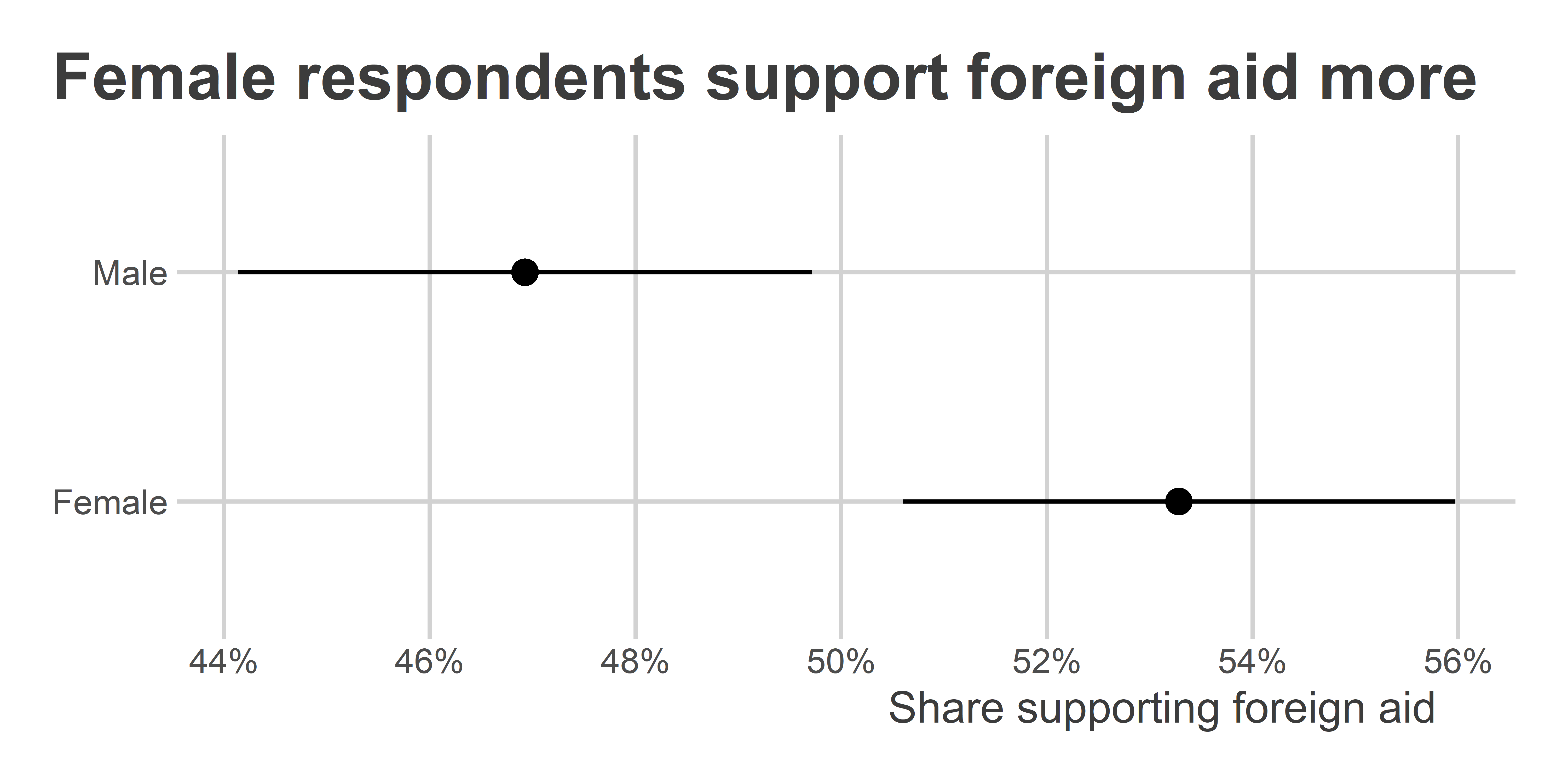
If you’re worried about this difference influencing the results, you can turn to a technique called block randomization, or what some researchers call stratified randomization. The idea is to randomize treatment within a specific group rather than across the whole data regardless of unit characteristics. In the case of gender and aid attitudes, a good strategy might be to block-randomize based on gender to ensure proportionate numbers of treated and control male and female respondents. You can do this with block_ra():
Data |>
  mutate(
    blockTr = block_ra(blocks = gender)
  ) -> Data
Check it out:
Data |>
  group_by(gender) |>
  count(blockTr)
# A tibble: 4 × 3
# Groups: gender [2]
gender blockTr n
<dbl> <int> <int>
1 0 0 309
2 0 1 309
3 1 0 335
4 1 1 336Compare this with what you got with simple random assignment. As you can see, there’s some notable discrepancies between the genders and treatment versus control conditions. Since gender clearly explains values of the outcome variable of interest, you could inadvertently generate misleading results about the treatment effect. But, by ensuring an equal number of males and females receive treatment, you can avoid this problem.
Data |>
  group_by(gender) |>
  count(simpleTr)
# A tibble: 4 × 3
# Groups: gender [2]
gender simpleTr n
<dbl> <int> <int>
1 0 0 297
2 0 1 321
3 1 0 351
4 1 1 320You can also block-randomize on multiple categories at the same time, say gender and race:
Data |>
  mutate(
    blockTr = block_ra(blocks = paste(gender, race3))
  ) -> Data
The beauty with this approach is that you can get really specific about how you want to, ahead of time, effectively control for different factors in your RCT. The main limitation with block-randomization, however, is that you can only block on factors that you can observe. If you’re concerned that variable X will influence your outcome and you want to be sure that you don’t get a disproportionate number of observations with characteristic X in either your control or treatment group, you should try really hard to ensure you collect data on X before you randomize.
All of this data that you collect about your observations is what you call pre-treatment data. You call it this because you collect information about it before you give treatment. Data collected after treatment is called post-treatment. This distinction seems trivial now, but when dealing with other kinds of research designs (such as selection on observables in the next chapter), you have to be careful about whether the factors you adjust for in your analysis are pre- or post-treatment.
9.3.4 Cluster Assignment
Cluster randomization involves randomizing, not at the level of individuals or within blocks, but instead at the level of groups or clusters.
A classic example of a clustered design is an experiment involving classrooms in a school. Some studies looking at the effect of curriculum or teacher characteristics follow a clustered research design for logistical reasons. It often is impossible to offer different students in the same classroom different interventions. How can you reasonably expect a teacher to give one lesson to half the class, and a different version of the lesson to the other? You can’t. Instead, researchers have to assign whole classrooms to different interventions. Sometimes they need to assign a treatment to an entire school.
The cluster_ra() function does cluster-randomization. Say you clustered treatment by education level in your foreign aid study. Here’s how you’d do it.
Data |>
  mutate(
    clusterTr = cluster_ra(clusters = educ)
  ) -> Data
Notice that individuals in different education categories have either all gotten treatment or all have been assigned to the control condition:
Data |>
  group_by(educ) |>
  count(clusterTr)
# A tibble: 6 × 3
# Groups: educ [6]
educ clusterTr n
<dbl> <int> <int>
1 1 1 42
2 2 0 467
3 3 1 296
4 4 1 122
5 5 0 228
6 6 0 134It practice, clustering on education would make no sense, but for the sake of showing how the function works, there you go.
You could also imagine that individuals who took your survey were from different cities and you could only implement your intervention at the level of cities, as would be the case with a public messaging intervention, for example. The below code simulates some cities your survey respondents might live in, and then it cluster-randomizes treatment by city.
Data |>
  mutate(
    city = sample(LETTERS[1:10], n(), T),
    clusterTr = cluster_ra(clusters = city)
  ) -> Data
If you summarize the data, you can see that the clustered treatment assignment worked:
Data |>
  group_by(city) |>
  count(clusterTr)
# A tibble: 10 × 3
# Groups: city [10]
city clusterTr n
<chr> <int> <int>
1 A 1 121
2 B 0 120
3 C 0 119
4 D 0 128
5 E 0 130
6 F 1 148
7 G 1 129
8 H 0 138
9 I 1 129
10 J 1 1279.4 Analyze How You Randomize
The average treatment effect (ATE) is a pretty simple estimator of causal effects. Just take the difference in means between treated and control groups. However, the process of estimating the ATE can become a little more involved depending on the kind of RCT you use in your study. For simple and complete randomization designs, a simple difference in means estimator is sufficient. However, for block and cluster randomized designs you need to do a few extra things to ensure you minimize bias or errors in your estimate of the ATE.
The rule of thumb is to analyze how you randomize. The following examples demonstrate how you would estimate the ATE depending on which kind of randomization approach you used.
9.4.1 Simple and complete randomization
This one is pretty easy. You can just use a simple linear model like so:
lm(aid ~ simpleTr, data = Data)
Call:
lm(formula = aid ~ simpleTr, data = Data)

Coefficients:
(Intercept)     simpleTr
    0.52160     -0.03879
You can do exactly the same with complete randomization:
lm(aid ~ completeTr, data = Data)
Call:
lm(formula = aid ~ completeTr, data = Data)

Coefficients:
(Intercept)   completeTr
    0.50827     -0.03827
This is really simple, right? Keep this in mind when or if you happen to be in a position to design an RCT in the future, because this kind of randomization is dead-simple to analyze.
In practice, I don’t recommend using lm() in your analysis, however. Instead, you should use lm_robust() from {estimatr}. You already know from previous chapters that this function automates the process of getting robust standard errors for regression estimates. When it comes to estimating the results form an RCT, there’s a special kind of standard error that you want to use. Remember in the last chapter that when you do inference for an experiment, you’re making an inference to potential outcomes rather than to a population or a data-generating process. I showed that this implies a special null hypothesis known as the “sharp” null.
There’s a standard error known as “HC2” that is consistent with this kind of inference, and you can get lm_robust() to estimate it for you. For example:
library(estimatr)
lm_robust(aid ~ completeTr, data = Data, se_type = "HC2")
Estimate Std. Error t value Pr(>|t|) CI Lower
(Intercept) 0.50827206 0.01516337 33.5197250 1.469285e-177 0.4785244
completeTr -0.03827206 0.03849268 -0.9942684 3.202792e-01 -0.1137874
CI Upper DF
(Intercept) 0.53801972 1286
completeTr 0.03724329 1286It’s really that simple. On to block randomization.
9.4.2 Block randomization
If you block-randomized, you can technically apply the same approach as above, but it is recommended that you instead calculate the average treatment effect within blocks. This technically is a weighted version of the ATE.
The value of accounting for blocks in the analysis becomes increasingly important to the extent that the blocks are of different sizes and individuals within blocks had different probabilities of being assigned to treatment.
The standard approach for some time was to add block fixed effects to your regression model, which can be done with lm_robust() like so:
lm_robust(aid ~ blockTr,
          fixed_effects = ~ gender,
          data = Data)
Estimate Std. Error t value Pr(>|t|) CI Lower CI Upper DF
blockTr -0.00320758 0.02783934 -0.1152175 0.9082907 -0.05782313 0.05140798 1285Note that this is equivalent to just writing the following with lm():
lm(aid ~ blockTr + gender, data = Data)
Call:
lm(formula = aid ~ blockTr + gender, data = Data)

Coefficients:
(Intercept)      blockTr       gender
   0.470859    -0.003208     0.063585
Essentially, the block fixed effects are control variables that you add to the model, and they’re indicators for the different blocks observations happen to be in.
While this approach can work, some research has shown that it can sometimes give inappropriate weights and actually bias your estimate of the ATE. The reason is that some blocks can be outliers, and the ATE for these blocks could drive up or down your estimate.
As an alternative, you can use a method called the Lin Estimator. This approach involves interacting the treatment with blocks or strata after mean centering them. It’s a technical read, but you can learn more about the justification of this approach from a 2013 study by Winston Lin where he proposes this method. The Lin estimator is also the approach that the US Office of Evaluation Sciences recommends as its default for block randomized studies (link: https://oes.gsa.gov/assets/files/block-randomization.pdf).
The model specification that this calls for can be annoying to write out, but the lm_lin() function from {estimatr} makes using the Lin Estimator easy. Just write:
lm_lin(aid ~ blockTr,
       covariates = ~ gender,
       data = Data)
Estimate Std. Error t value Pr(>|t|) CI Lower
(Intercept) 0.503979618 0.01959910 25.7144269 5.759272e-118 0.46552984
blockTr -0.003207842 0.02780142 -0.1153841 9.081587e-01 -0.05774904
gender_c 0.122744802 0.03922920 3.1289146 1.794030e-03 0.04578445
blockTr:gender_c -0.118150488 0.05564936 -2.1231238 3.393434e-02 -0.22732415
CI Upper DF
(Intercept) 0.542429392 1284
blockTr 0.051333358 1284
gender_c 0.199705157 1284
blockTr:gender_c -0.008976827 1284The estimate for blockTR is the estimate of the ATE based on this Lin estimator. This is the default option you should consider for block-randomized trials.
9.4.3 Cluster randomization
When you use a cluster -randomized design, you don’t need to add special fixed effects, but you do need to change the way you calculate your standard errors. The reason is that uncertainty that comes from random assignment is not at the individual level but at the level of clusters. To make causal inferences with the sharp null as your reference point, you are trying to imagine what different sets of ATEs you could have estimated by giving treatment to different units. In a cluster randomized trial you didn’t just give treatment to different units; you gave it to different groups of units. So when you make an inference to the sharp null, you want to consider what set of ATEs you could have gotten by assigning treatment to different groups (not just individuals).
That means that you want your standard errors to capture uncertainty, not from shaking up which individuals got treatment, but instead by shaking up which clusters got treatment. To ensure you do this, you can cluster the HC2 standard errors by the groups you cluster randomized with. It’s quite easy to do with lm_robust() using the cluster option. Here’s an example with the clustered treatment that you assigned by hypothetical cities in the data:
lm_robust(aid ~ clusterTr, data = Data, clusters = city) Estimate Std. Error t value Pr(>|t|) CI Lower
(Intercept) 0.49448819 0.02297305 21.5247102 0.0000283398 0.43061567
clusterTr 0.01546587 0.02727029 0.5671326 0.5862534156 -0.04747174
CI Upper DF
(Intercept) 0.55836071 3.985895
clusterTr 0.07840347 7.9620539.5 The ITT and CATE
Sometimes people don’t comply with your experimental designs. This can influence the results of your studies, but under the right conditions, you can adjust for noncompliance.
People can fall into one of four different categories:
- Compliers: People that follow the treatment given.
- Always-takers: People that always are treated no matter their assignment.
- Never-takers: People that never are treated no matter their assignment.
- Defiers: People that always do the opposite of what they are assigned.
There’s a classic get-out-the-vote experiment that will help make these scenarios concrete. Here’s code to get the relevant data:
url <- "https://raw.githubusercontent.com/milesdwilliams15/Teaching/main/DPR%20201/Data/GOTV_Experiment.csv"
gotv <- read_csv(url)
glimpse(gotv)
Rows: 50,000
Columns: 9
$ female <dbl> 0, 1, 0, 1, 0, 0, 1, 0, 0, 0, 0, 0, 0, 0, 0, 0, 1,…
$ age <dbl> 34, 37, 43, 45, 47, 45, 57, 20, 30, 25, 36, 27, 25…
$ white <dbl> 1, 0, 1, 1, 0, 1, 1, 1, 1, 0, 1, 0, 0, 1, 1, 0, 0,…
$ black <dbl> 0, 0, 0, 0, 1, 0, 0, 0, 0, 1, 0, 1, 0, 0, 0, 0, 1,…
$ employed <dbl> 1, 1, 1, 0, 1, 0, 1, 1, 0, 1, 1, 1, 1, 0, 1, 0, 1,…
$ urban <dbl> 1, 0, 0, 0, 0, 0, 1, 1, 0, 0, 0, 0, 0, 1, 1, 1, 1,…
$ treatmentattempt <dbl> 0, 1, 1, 1, 0, 1, 0, 0, 1, 1, 0, 1, 1, 0, 1, 0, 0,…
$ successfultreatment <dbl> 0, 1, 1, 0, 0, 0, 0, 0, 0, 0, 0, 1, 1, 0, 1, 0, 0,…
$ turnout <dbl> 1, 0, 1, 0, 1, 1, 1, 0, 1, 0, 0, 0, 0, 0, 1, 0, 1,…In this study, individuals were randomly assigned to get a phone call urging them to go out and vote. This was fielded in New Haven, CT during the 1998 mid-term elections.
This study had a problem. Not all individuals in the data who were randomly assigned to get a get-out-the-vote phone call actually picked up the phone. To put a precise number on it:
complied <- mean(gotv$successfultreatment[gotv$treatmentattempt==1])
complied
[1] 0.7688753That comes out to a 77% compliance rate with the treatment.
This will bias the results against finding a significant treatment effect, but you can use non-compliance information to recover a special kind of causal estimate called the compliers average treatment effect or CATE which corrects for this issue. To calculate it, you first need to calculate something else called the intention to treat effect or ITT.
The ITT is calculated the same as the ATE, but since you know that you have noncompliers in the data the estimate has a conceptually different interpretation:
ITT <- coef(lm(turnout ~ treatmentattempt, gotv))[2]
ITT
treatmentattempt
0.07098882 The ITT is the product of a couple of different things: (1) the compliance rate and (2) the CATE: \[\text{ITT} = c \times \text{CATE}\]
Using some simple algebra, you can take your known ITT and the known compliance rate c to recover the CATE estimate. \[\text{CATE} = \frac{\text{ITT}}{c}\]
So in R you would just write:
CATE <- ITT / complied
CATE
treatmentattempt
0.09232814 You can get this same estimate using regression. Specifically, using instrumental variables regression. This approach involves a two-stage process of arriving at the CATE. The function iv_robust() from {estimatr} takes care of these steps for you. You just need to give it a slightly different way of writing a formula than you’ve done up to now:
iv_robust(turnout ~ successfultreatment | treatmentattempt,
          data = gotv)
Estimate Std. Error t value Pr(>|t|) CI Lower
(Intercept) 0.48467348 0.003176074 152.60146 0.000000e+00 0.47844834
successfultreatment 0.09231023 0.005788652 15.94676 4.159227e-57 0.08096441
CI Upper DF
(Intercept) 0.4908986 49740
successfultreatment 0.1036561 49740See how the coefficient for successfultreatment is identical to the one you previously calculated.
Notice that this isn’t the same thing as just doing this:
lm_robust(turnout ~ successfultreatment,
          data = gotv)
Estimate Std. Error t value Pr(>|t|) CI Lower
(Intercept) 0.4742721 0.002857794 165.95741 0.000000e+00 0.4686707
successfultreatment 0.1192421 0.004552561 26.19231 3.412514e-150 0.1103190
CI Upper DF
(Intercept) 0.4798734 49740
successfultreatment 0.1281652 49740To show what’s going on here, I’ll use lm() and break the process down. It involves two stages.
In stage 1, you first need to estimate the relationship between treatment assignment and treatment compliance:
stage1_fit <- lm(successfultreatment ~ treatmentattempt, gotv)There should be a significant relationship between the two:
summary(stage1_fit)
Call:
lm(formula = successfultreatment ~ treatmentattempt, data = gotv)

Residuals:
    Min      1Q  Median      3Q     Max
-0.7689  0.0000  0.0000  0.2311  0.2311

Coefficients:
                  Estimate Std. Error t value Pr(>|t|)
(Intercept)      1.199e-13  1.893e-03     0.0        1
treatmentattempt 7.689e-01  2.671e-03   287.8   <2e-16 ***
---
Signif. codes:  0 '***' 0.001 '**' 0.01 '*' 0.05 '.' 0.1 ' ' 1

Residual standard error: 0.2987 on 49998 degrees of freedom
Multiple R-squared:  0.6236,    Adjusted R-squared:  0.6236
F-statistic: 8.283e+04 on 1 and 49998 DF,  p-value: < 2.2e-16
In stage 2, you’ll do something clever. Rather than look at the relationship between successful treatment and turnout, you’ll look at the relationship between predicted successful treatment and turnout:
stage2_fit <- lm(turnout ~ predict(stage1_fit), gotv)
summary(stage2_fit)
Call:
lm(formula = turnout ~ predict(stage1_fit), data = gotv)

Residuals:
    Min      1Q  Median      3Q     Max
-0.5557 -0.4847  0.4443  0.4443  0.5153

Coefficients:
                    Estimate Std. Error t value Pr(>|t|)
(Intercept)         0.484673   0.003167  153.04   <2e-16 ***
predict(stage1_fit) 0.092328   0.005812   15.88   <2e-16 ***
---
Signif. codes:  0 '***' 0.001 '**' 0.01 '*' 0.05 '.' 0.1 ' ' 1

Residual standard error: 0.4983 on 49740 degrees of freedom
  (258 observations deleted due to missingness)
Multiple R-squared:  0.005048,  Adjusted R-squared:  0.005028
F-statistic: 252.3 on 1 and 49740 DF,  p-value: < 2.2e-16
This coefficient is identical to the CATE you got before.
Importantly, the standard error from this approach is incorrect. The reason is that the first-stage predictions used in the second-stage model are estimates. That means that classical OLS standard errors (or standard robust standard errors) aren’t going to capture all the relevant uncertainty in the data. Thankfully, iv_robust() takes care of this and reports the correct standard errors.
Another nice feature of the regression approach to estimating the CATE is that it can accommodate controlling for covariates. For example, say you want to account for urban/rural status as you estimate the CATE. you can specify your regression model as follows:
iv_robust(turnout ~ successfultreatment + urban | treatmentattempt + urban,
          data = gotv)
Estimate Std. Error t value Pr(>|t|) CI Lower
(Intercept) 0.52966399 0.005518537 95.979063 0.000000e+00 0.51884759
successfultreatment 0.04842280 0.007313844 6.620704 3.611159e-11 0.03408758
urban -0.05639415 0.005625235 -10.025207 1.243799e-23 -0.06741967
CI Upper DF
(Intercept) 0.54048038 49739
successfultreatment 0.06275802 49739
urban -0.04536862 49739Note that you must include the same covariates on both sides of the | that you want to control for.
9.6 Checking Balance and (Non)Random Attrition
Sometimes in your studies, experiments break. This was certainly the case in the above experiment. A sign that something has gone wrong is when treatment and control groups differ substantially on observed covariates. This is known as balance.
To assess balance quickly, you can get lm_robust() to tell you how much your covariates differ by treatment. Notice the use of cbind() on the left-hand side of the equation. This code forces lm_robust() to report the average difference in each of the covariates specified inside cbind() based on treatment. It then pipes the data into some code that produces a coefficient plot based on the results.
## First, regress each covariate on treatment assignment
lm_robust(cbind(female, age, white,
                black, employed, urban) ~ treatmentattempt,
          data = gotv) |>
  ## tidy the results
  tidy() |>
  filter(term != "(Intercept)") |>
  ## plot
  ggplot() +
  aes(x = estimate,
      xmin = conf.low,
      xmax = conf.high,
      y = outcome) +
  geom_pointrange(size = .1) +
  geom_vline(xintercept = 0, lty = 2) +
  labs(x = "Difference relative to control",
       y = NULL,
       title = "Covariate Balance between Treatment and Control")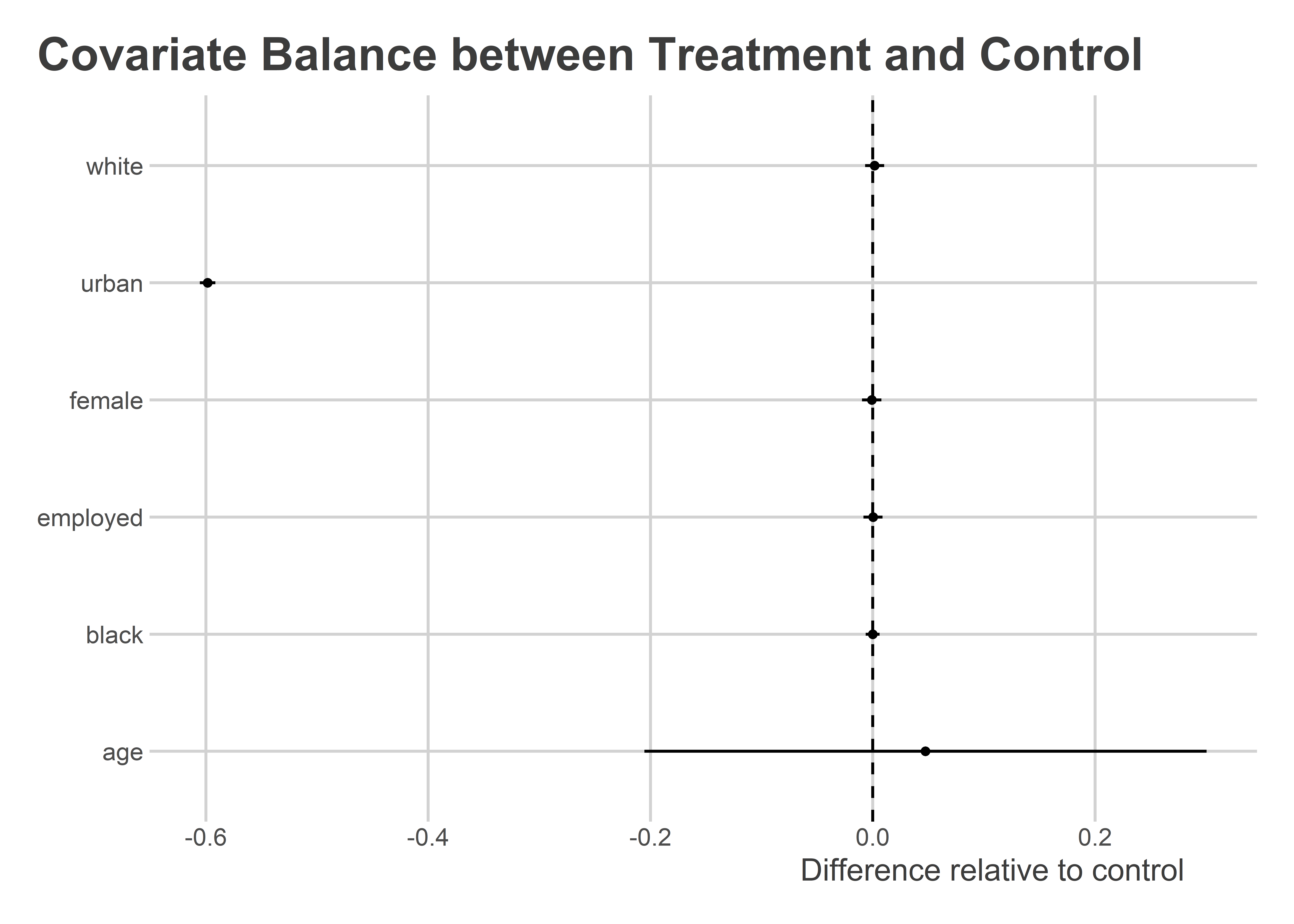
It looks like people in urban settings were unusually unlikely to be in the treatment condition. If urban status is important for predicting turnout (which it is), that’s a problem.
Attrition can be a problem in experiments, too. In this same experiment, you have missing data for 258 individuals regarding whether they turned out to vote. Is missingness correlated with other characteristics of respondents? Yes. Both non-white and younger respondents were more likely to have missing values for turnout. This could also bias estimates for the effect of the GOTV campaign.
lm_robust(
  is.na(turnout) ~ female + age + white + black + employed + urban,
  data = gotv
) |>
  tidy() |>
  filter(term != "(Intercept)") |>
  ggplot() +
  aes(x = estimate,
      xmin = conf.low,
      xmax = conf.high,
      y = term) +
  geom_pointrange(size = .1) +
  labs(x = "Coefficient",
       y = NULL,
       title = "Who has missing turnout data?") +
  geom_vline(xintercept = 0,
             lty = 2)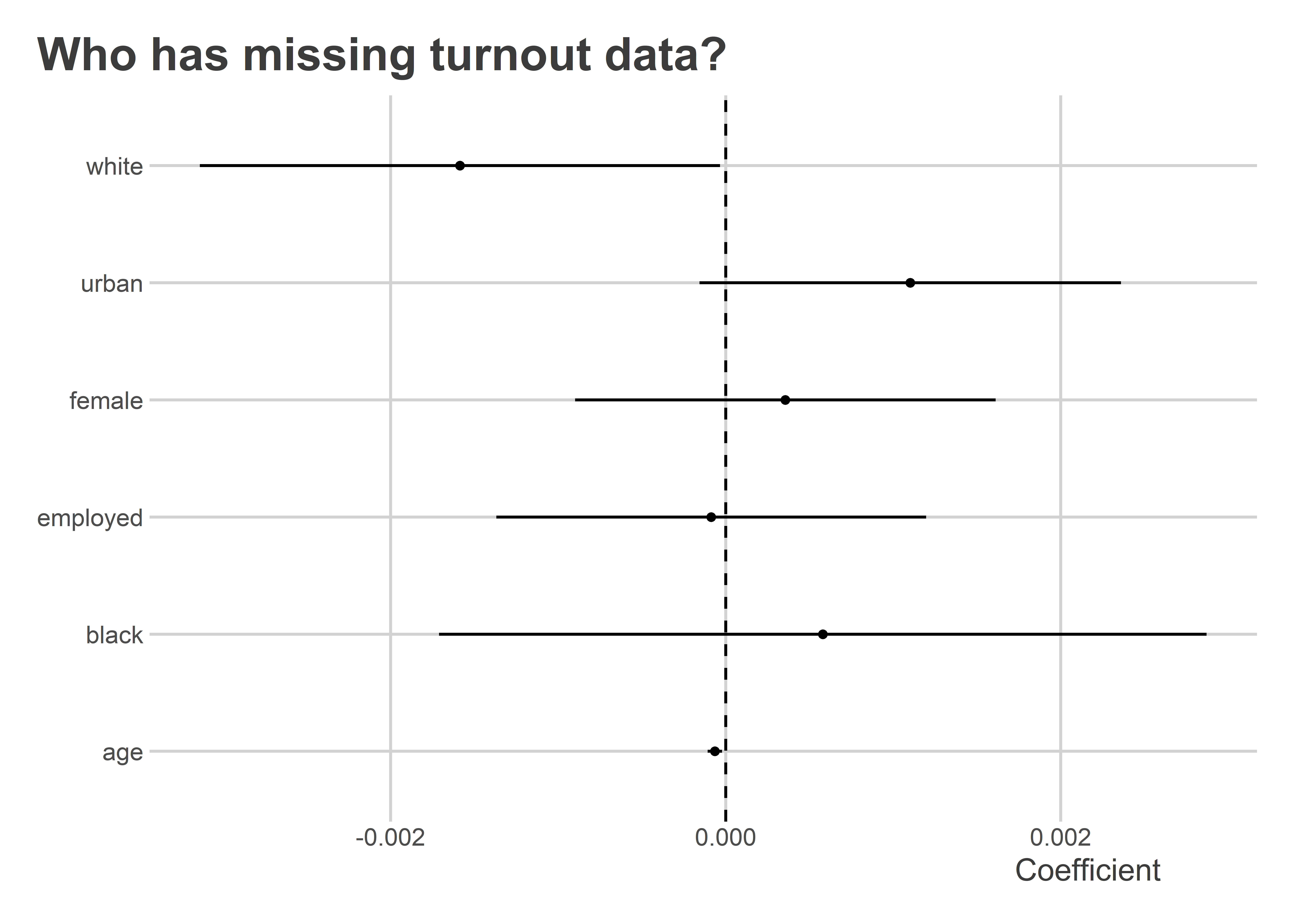
9.7 I barely scratched the surface
There is so much more that I could discuss with respect to RCTs. But you have to learn to crawl before you can run, and the above discussion has already provided plenty to think about.
The main things you need to remember are:
RCTs help you make causal claims by ensuring treatment assignment is independent of potential confounders
You can randomize a variety of different ways depending on your needs
How you randomized will determine how you analyze
Experiments can break, but there are techniques for handling that