## Open the {tidyverse}
library(tidyverse)

## Set the seed so results are replicable
set.seed(123)

## Simulate potential and revealed outcomes
tibble(
  # values without treatment
  Y0 = rnorm(100),

  # values with treatment
  Y1 = 1/2 + Y0,

  # treatment assignment
  D = rep(0:1, each = 50) |>
    sample(),

  # reveal outcomes
  Yobs = Y1 * D + Y0 * (1 - D)
) -> Data8 Causation
8.1 Goals
Learning objectives:
- Introduce the concept of potential outcomes.
- Explain the fundamental problem of causal inference.
- Introduce the sharp null hypothesis.
8.2 From Correlation to Causation
Descriptive and predictive research designs, which I discussed in previous chapters, are all about measuring correlations in observational data. For descriptive studies, the goal is to document basic facts about the world. For predictive studies, the goal is to use correlations observed in the past to predict events in the future.
In causal research designs (the subject of this chapter and the rest of these lecture notes) the goal is to measure correlations in data, too. But that isn’t all. Claiming that a correlation exists between two factors is one thing. Demonstrating that this correlation exists because two factors are causally related is something else entirely. The stakes are much higher.
When I, as a researcher, want to claim that some factor causes another, I’m making a claim about how the world works. Someone, say a policy-maker, might try to manipulate the causal factor I identified in my study in order to effect some desired outcome for society because they believe my causal claim.
You can think of causal research as prescriptive. If I say that, for example, mandatory masking policies save lives during a pandemic, I’m going beyond the mere claim that masking is correlated with lower mortality. I’m saying that if you mandate masking, it will lead to lower mortality. In short, causal research implies that if you do \(X\), then \(Y\) will happen.
Because causal research has the potential to be prescriptive, this demands great care and responsibility on the part of researchers to ensure their causal claims are based on sound data and research methods. If you aren’t careful, you could end up recommending a (potentially expensive) policy that isn’t actually efficacious. You might also recommend against using a policy that works.
So how do you know if a policy intervention is a good idea? This kind of public policy question is an important area of research within political science, and other fields like economics and public administration. In this, and the coming chapters, I’ll talk about the challenges of causal inference and a variety of research designs for identifying causal relationships across a wide range of scenarios. Specifically, I’ll talk about the gold standard of causal research (the randomized controlled trial) and other causal research designs that offer a next-best option when the gold standard isn’t feasible.
But first, it’s worth spending some time talking about causation conceptually. While it seems simple, it actually is both technically and philosophically profound. Making causal claims requires some strong assumptions about the world, not just as you observe it by way of data, but also as you might have observed it under different circumstances. This means you need to take seriously the concepts of potential outcomes and counterfactuals. I’ll talk about those next.
8.3 The Potential Outcomes Framework
The potential outcomes framework is central to the problem of causal inference. It centers around the idea that for any set of outcomes you observe, there are other outcomes that could have potentially occurred that you don’t observe. I think a simple simulation will help explain.
The below R code generates a hypothetical dataset. There is an outcome \(Y\) that is just a random, normally distributed variable. There is also a causal variable \(D\) (you could call this the “treatment” variable) that affects the values of \(Y\). The unique thing about this factor is that it reveals the values of the outcome variable. In the below dataset, there are two versions of the outcome. One is if there is no exposure to the treatment, and another is if there is exposure. In revealing outcomes, only some observations in the data get exposed to the treatment so that the observed outcomes are a mix of values with and without treatment. But here’s the twist, for any one observation, you can only see one of its potential outcomes. Either you see what \(Y\) looks like for a given observation with treatment, or without. It’s never both.
The fact that you can’t observe all potential outcomes is the fundamental problem of causal inference. At best, you only observe half of the data that you need to calculate the true causal effect of some intervention. If you could observe all potential outcomes, estimating a causal effect would be easy. For instance, in R all you would need to do is take the mean difference between potential outcomes with treatment and without, and this would tell you the average treatment effect (ATE):
## estimate the average treatment effect
ate <- mean(Data$Y1 - Data$Y0)

## report its value
ate
[1] 0.5In the data that I simulated, I specified that the outcome with treatment for each observation would be exactly one half greater than without treatment. Sure enough, when I calculate the average difference between potential outcomes with and without treatment, the average treatment effect, or ATE, comes out to this precise value.
But, as Dwight Schrute says in The Office, “[i]f ‘onlys’ and ‘justs’ were candies and nuts, then every day would be Erntedankfest.” You can’t observe all potential outcomes. You therefore cannot, in reality, directly calculate the ATE. So, what to do instead?
Under very particular conditions, it is possible to estimate the ATE using only observed outcomes by taking the mean of the outcome among those who got treatment, the mean of the outcome among those who didn’t, and calculating the difference. In R, this would look like:
## calculate the estimated ATE
est_ate <- mean(Data$Yobs[Data$D == 1]) - mean(Data$Yobs[Data$D == 0])

## report the estimate
est_ate
[1] 0.5042286Note that the estimate isn’t identical to the true ATE of one half. It’s close, though. Very close. This isn’t just due to dumb luck, by the way. There’s a reason this estimate is so close to the truth, which I’ll discuss more in the next section.
8.4 Identifying Good Counterfactuals
At the heart of causal research is the task of making good comparisons using the data you observe to get an approximation of unobserved potential outcomes. This task is both an art and a science because it often requires as much creativity as it does methodological rigor. The counterfactuals you generate with your research design provide a window into what outcomes might have been for treated and non-treated (control) observations if their treatment exposure had been different.
Ideal counterfactuals are observations that are otherwise similar to each other, except for their exposure to treatment. To have valid counterfactuals, however, treatment exposure must be completely independent of any of the characteristics of the observations in your data. This can only be true if treatment assignment is random.
If treatment status is determined by factors that also predict your outcome of interest, this poses a challenge. It makes it hard to know if observations differ in their outcomes because of the treatment or because of some other factor. This is the problem of confounding that I talked about in the context of descriptive research and U.S. foreign aid cuts. The problem of confounding is even more troublesome in causal research where the goal is to offer sound policy advice. Say you wanted to test a new reading curriculum for grade schoolers to see if it improves reading scores, but the schools you fielded this new curriculum in were in disproportionately affluent districts. This would make it really hard to compare the average of the treated school reading scores with the average of non-treated school reading scores and claim that any difference in reading ability is due to the new curriculum. The average reading score in more affluent school districts is likely to be higher than in more impoverished districts due to factors besides the new curriculum. So how can you know if the curriculum really worked, had no effect, or actually made reading scores worse? The answer is that you can’t.
The solution to this problem is to make sure that exposure to treatment is random. This is the reason why the estimated ATE I calculated in the last section was so close to the true ATE. When I assigned treatment status to observations in the data, I did so at random (that’s what the sample() function allowed me to do in my R code). As a result, nothing particular to any one observation made it more or less likely to get treated. All units of observation had an equal chance of getting treated, and it was the luck of the draw that determined their ultimate treatment status.
Random treatment assignment is what guarantees good counterfactuals, at least in expectation (that is, on average across repeated trials). When treatment status is random, it is possible to simply take the difference in means between treated and non-treated groups because these groups are, by default, ideal counterfactuals. Consider the below simulation that takes the potential outcomes I generated in the last section and then repeatedly re-assigns treatment, revealing new outcomes. Notice that there’s variation in the estimated ATEs but that, on average, these estimates cluster around the truth.
## map_dfr() will iterate a process across whatever
## values you give it in .x and return a data frame
## with outputs stored in a single column with a
## unique row per iteration. In the below code
## I use it to repeat the process of shuffling
## treatment assignment, revealing observed
## outcomes, and estimating the ATE
map_dfr(
  .x = 1:2000,
  .f = ~ Data |>
    mutate(
      D = sample(D),
      Yobs = Y1 * D + (1 - D) * Y0
    ) |>
    summarize(
      est_ate = mean(Yobs[D == 1]) -
        mean(Yobs[D == 0])
    )
) -> sim_ates

## Visualize the distribution with a histogram.
ggplot(sim_ates) +
  aes(est_ate) +
  geom_histogram(
    fill = "gray",
    color = "black"
  ) +
  geom_vline(
    xintercept = 0.5,
    linewidth = 1,
    color = "navy"
  ) +
  labs(
    title = "Simulated ATE estimates",
    subtitle = "Estimates simulated based on random treatment reassignment",
    x = "Estimated ATEs",
    y = "Frequency"
  ) +
  scale_x_continuous(
    breaks = c(0, .5, 1),
    labels = c("0", "True ATE", "1")
  )
`stat_bin()` using `bins = 30`. Pick better value `binwidth`.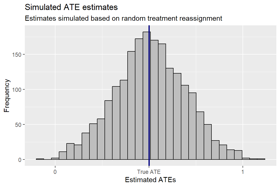
The fact that random treatment assignment buys you good counterfactuals in expectation is worth considering a bit more. Even though treated and control groups will be similar on average, there’s always a chance that you’ll end up with bad counterfactuals anyway. This is why even the best causal research study is never the last word on a causal relationship. Often you need to conduct multiple studies to better assess the effect of a given policy. As the above simulated results show, even though on average random treatment assignment gives you an estimated ATE very close to the truth, there are some scenarios where the estimated ATE is close to 0 and others where the estimate is almost double the size of the true ATE. Imagine that a single study is like taking one random draw from this distribution of possible ATE estimates. Odds are pretty good that your study will be close to the truth, but there’s also a good chance that you might be way off. This is why no single causal study can settle debates about good policy.
8.5 Quantifying Uncertainty about Causal Effects
The fact that there can be so much variation in estimated treatment effects is why it’s important to take uncertainty into account in causal research, just as it is with descriptive and predictive studies. However, when doing causal inference, particularly in cases where you assign treatment randomly, the kind of inference that you want to do is a bit different.
When I introduced statistical inference in the first part of this book, I did so using bootstrapping. The idea is that you assume that the data you observe is one among many possible versions of it you could have drawn from a population or from some historical data-generating process. By taking re-samples with replacement from your existing data, it simulates the variation you’d expect to see in the data from one hypothetical re-draw to the next.
For causal research, when treatment is assigned at random, you also want to quantify the variation you’d expect to see in estimated treatment effects if you could repeat your study multiple times, but bootstrapping (or some analogous analytical solution) isn’t the right approach to calculate this variation. Instead, you need a method that lets you calculate variation due to treatment assignment specifically. The reason is that you aren’t interested in making an inference to a population or to a historical data-generating process. You’re interested in making an inference to potential outcomes.
When you make this inference, you also usually have a hypothesis test in mind. Recall that this is also important for doing descriptive research where you want to test against the assertion that no true correlation exists between factors in your data. In the case of causal inference, the null hypothesis is simply that the causal variable in question has no effect on the outcome variable.
This version of the null hypothesis has a very special interpretation. It’s called the sharp null hypothesis. This particular version of the null was introduced by the statistician Sir Ronald Fisher 90 years ago, and it holds that there is absolutely no difference between potential outcomes with and without treatment. It asserts, not just that the average difference due to treatment is zero, but that on a case-by-case basis the difference due to treatment is zero.
To better talk about what this implies, it’ll be useful to introduce some notation. First, let \(Y_{0i}\) represent the value of some outcome variable for an observation \(i\) if \(i\) doesn’t get exposed to a causal variable \(D_i\). Further, let \(Y_{1i}\) represent this outcome for \(i\) if it does get exposed to treatment. Often, researchers use the Greek letter \(\delta\) to represent the difference in an outcome due to treatment. You can specify this difference for observation \(i\) as:
\(\delta_i = Y_{1i} - Y_{0i}\)
Under the sharp null hypothesis, you assert that \(\delta_i = 0\) \(\forall\) \(i\). In plain terms, you claim that this difference between potential outcomes is zero for every single observation (\(i\)) in your data.
Now, as I already discussed, you can’t actually test this null hypothesis directly since you can’t observe both \(Y_{0i}\) and \(Y_{1i}\) at the same time. By assigning treatment to \(i\) you observe only one of these potential outcomes. So in practice, the actual estimate you get from a causal study that you then compare against the sharp null is:
\(\hat \delta = \frac{\sum_i Y_i(D_i = 1)}{m} - \frac{\sum_i Y_i(D_i = 0)}{n - m}\)
In words, your estimate of the difference due to treatment, represented by \(\hat \delta\) is the average of all revealed outcomes for \(m\) number of individuals who got treatment, minus the average of all revealed outcomes for \(n - m\) individuals who didn’t. If the sharp null is true, you would expect \(\hat \delta = 0\).
In practice, however, even if it really is true that \(\delta_i = 0\), it is still possible to observe a \(\hat \delta \neq 0\). The reason is that in randomly assigning treatment and then estimating the ATE, it’s quite possible to get a non-zero estimate for the ATE due to dumb luck because of chance differences in the outcome from one individual to the next.
Here’s where the magic of the sharp null comes into play. Because it asserts that \(\delta_i = 0\), and hence that potential outcomes with or without exposure to treatment are identical, it is possible to shuffle treatment assignment again and again and again and re-estimate the ATE. This will give you a distribution of possible values of \(\hat \delta\) that you would get if the sharp null hypothesis is true.
What’s greater still is that you can compare your original ATE estimate to this distribution under the sharp null to calculate how unlikely your observed estimate is assuming the sharp null is true. In short, you can calculate a \(p\)-value.
The below code implements some R code to make this happen with the data I simulated earlier. First, I calculate the ATE for the observed values of the outcome variable. Second, I shuffle treatment status multiple times (1,000) and re-estimate the ATE. Third, I calculate the proportion of the time that the original ATE estimate is as extreme as the simulated ATE estimates under the sharp null. This is my \(p\)-value. In this particular example, the \(p\)-value is quite small. Just like with conventional hypothesis testing, the tradition is to reject the sharp null if the \(p\)-value is less than 0.05. Based on the results below, it looks like you can reject the sharp null.
## First, estimate the ATE
est_ate <- Data |>
  summarize(
    est_ate = mean(Yobs[D == 1]) -
      mean(Yobs[D == 0])
  )

## Second, re-estimate the ATE by shuffling Tr
nul_ate <- map_dfr(
  .x = 1:1000,
  .f = ~ Data |>
    mutate(D = sample(D)) |>
    summarize(
      nul_ate = mean(Yobs[D == 1]) -
        mean(Yobs[D == 0])
    )
)

## Third, calculate the probability of the original
## ATE estimate if the sharp null is true.
nul_ate |>
  summarize(
    est_ate = est_ate$est_ate,
    p.value = 2 * pmin(
      mean(est_ate > nul_ate),
      mean(est_ate < nul_ate)
    )
  )
# A tibble: 1 × 2
est_ate p.value
<dbl> <dbl>
1 0.504 0.0088.6 What’s to Come
I’ve only begun to scratch the surface of causal research. In the coming chapters I’ll talk about four different research designs for making causal inferences. In order: randomized controlled trials, selection on observables, regression discontinuity, and difference-in-differences.
I’ll also introduce relevant R code for implementing these methods. Rest assured that the verbose code I used in this chapter isn’t necessary. I used a less elegant approach because I think it’s important to understand the mechanics of causal inference before you use more conventional tools that tend to obscure these mechanics, or keep them hidden entirely.
The linear regression model will make an appearance with each of the four research designs I’ll talk about. The key difference in each approach will be in how these regression models are specified and how the results are interpreted. I’ll also introduce you to a new kind of robust standard error that’s appropriate for randomized treatment assignment.
As I cover these research designs, I’ll also talk about some common mistakes and pitfalls. For methods other than randomized controlled trials, you have to be careful about your approach and your interpretation of the results. Even for randomized trials there are factors you need to pay attention to. Not all randomized studies randomize in the same way. How you randomize treatment can make a big difference. I’ll take up this issue and more related to randomized trials in the next chapter.