library(tidyverse)
library(estimatr)
library(rddtools)
data(house) # attaches the house data11 Regression Discontinuity
11.1 Goals
Learning objectives:
- Controlling for covariates in a selection on observables or SOO design using a multiple regression model is one way to recover causal estimates from non-experiments.
- But SOO designs are notoriously susceptible to omitted variable bias and a host of other challenges.
- In some settings you can exploit certain facts about how data were generated to make more reliable causal inferences.
- One such approach is to use an arbitrary discontinuity in some data to estimate a local average treatment effect or LATE.
- When you do this, you are using a regression discontinuity design or RDD.
11.2 Introduction to regression discontinuity designs
A regression discontinuity design (RD) is known as a quasi-experimental design (QED). Studies that use QEDs work by identifying something seemingly random, or more often arbitrary, about how units of observation got exposed to a causal variable. In RDs, this is usually a threshold, such as an income requirement for receiving a government benefit. The idea is that observations at or near this threshold should be alike, which means you can compare outcomes among those just before and after this threshold to determine if a policy had any effect on those exposed to it.
This kind of design can be very effective, and the results typically are trusted a bit more than selection on observable (SOOs) designs, which I discussed in the last chapter. But RDs do have one big limitation. The observations at or near the threshold for getting exposed to the causal variable are the best counterfactuals for estimating the average treatment effect (ATE) of a policy or other intervention. That means the evidence of a causal effect is local to the point of the discontinuity. The term “local” is a technical term that researchers use to clarify that an effect from an RD can’t be generalized to other data points far away from the threshold. An RD that tests whether access to a government benefit has a causal effect on particular outcomes can only estimate the causal effect for observations at or near the threshold for qualifying for the benefit. For this reason, you call the treatment effect from an RD a local average treatment effect (LATE).
The way the LATE is estimated in a regression analysis is a bit more involved than with SOOs. To calculate it, you need to estimate an interaction model. An interaction model lets the effect of one variable depend on the value of another, and it works by including the two relevant explanatory variables in the model equation, along with their product. This would be specified something like this:
\[ y_i = \beta_0 + \beta_1 x_i + \beta_2 z_i + \beta_3 (x_i \times z_i) + \epsilon_i \]
In this kind of model, the regression estimates for the explanatory variables have a new conditional interpretation. The estimate for the coefficient on \(x_i\) of \(\hat \beta_1\) isn’t just the average change in \(y_i\) given a change in \(x_i\). It’s the average change in \(y_i\) given a change in \(x_i\) when \(z_i = 0\). For any value of \(z_i \neq 0\), the overall relationship between \(x_i\) and \(y_i\) can potentially change. In fact, here’s what the more complex conditional relationship looks like for \(x_i\) and \(y_i\):
\[ \text{effect of x on y} = \beta_1 + \beta_3 z_i \]
The estimated coefficient of \(\hat \beta_3\) influences how the effect of \(x_i\) changes given the level of \(z_i\). For this reason, you call \(\beta_3\) an interaction effect, because it captures how values of \(z_i\) interact with \(x_i\) in predicting \(y_i\).
RDs generally rely on this same framework to estimate the LATE. At minimum, an RD model requires the following variables in your data:
- An outcome
- A treatment (usually this is binary)
- A (semi-)continuous running variable that determines treatment assignment
The interaction model the RD design relies on involves interacting the treatment indicator with the running variable, like so:
\[ \text{Outcome}_i = \beta_0 + \beta_1 \text{Treatment}_i + \beta_2 \text{Running-Var}_i + \beta_3 (\text{Treatment}_i \times \text{Running-Var}_i) + \epsilon_i \]
The “local” part of the LATE enters the equation by way of conditioning the effect of the treatment on the running variable being held constant at the threshold (discontinuity) that determines who gets treated. In short, the LATE equals:
\[ \text{LATE} = \beta_1 + \beta_3 \text{Running-Var}_i( = \text{Threshold}) \]
11.3 An example using U.S. House data
Consider some U.S. House incumbency data that you can access in R using the package {rddtools}. This data comes from a paper published by Lee (2008) to test whether U.S. House members enjoy an incumbency advantage. Incumbents are people who already hold an elected office and are running for re-election. The incumbency advantage is the idea that incumbents get an electoral boost simply because they are running for re-election rather than for the first time. This is either due to better name recognition or access to more resources by virtue of holding office. An RD design can help you test this theory.
You’ll need to install {rddtools}, Then you can write the following code to access the data. Open {tidyverse} and {estimatr} while you’re at it.
The dataset has two columns, x and y, that correspond to the Democratic vote margin in year t (column x) and the Democratic vote share in year t+2 (column y). If x < 0, then a candidate lost the previous election. If x \(\geq\) 0, then a candidate won the last election and, hence, is an incumbent.
You have all the building blocks you need to implement an RD. But first I should probably discuss why you need an RD to test the incumbency advantage in the first place.
The big question you should ask yourself is whether being an incumbent is correlated with other factors that might give a candidate an electoral boost. The answer is probably yes. Perhaps a candidate is uniquely popular, or maybe a congressional district is a historical stronghold for a particular party. Both of these factors would explain why a candidate won in a previous election and also why they can expect to win in the next. Therefore, the raw estimate of the effect of being an incumbent is probably going to be subject to omitted variable bias.
However, there are always little random differences from one election to the next. The weather could be better in one election versus the previous. Different issues may be salient. A scandal could have surfaced. Anything! The beauty of RDs is that they give you a way to leverage all of these little sources of random variation to get around omitted variable bias. This works by identifying the precise threshold needed for an observation to be “treated” with incumbency. That is precisely the point between winning an election with a majority of the vote, or just failing to reach this threshold, in the previous election. By estimating the effect of incumbency right at the threshold needed to win, you can get a reliable estimate of incumbency’s causal effect on future election performance.
Here’s the model you need to estimate:
\[ \text{Vote Share}_{it+2} = \beta_0 + \beta_1 \text{Incumbent}_{it} + \beta_2 \text{Vote Margin}_{it} + \beta_3 \left(\text{Incumbent}_{it} \times \text{Vote Margin}_{it} \right) + \epsilon_{it+2} \]
The outcome variable is the vote share for the Democratic Party in a future election. The predictor variables in the model include a binary indicator for whether the Democratic Party is the incumbent party (the causal variable of interest) and a continuous measure of the Democratic Party’s vote margin in the previous election. Conveniently, the point at which the vote margin equals zero is also the point of the discontinuity that determines incumbency. That means you can just use the value of \(\beta_1\) as the LATE since, by default, this estimate equals the effect of incumbency when the vote margin is zero.
Below is the code to estimate this model with the data. I’m using the lm_robust() function and having it return HC1 robust standard errors. As I discussed in the last chapter, when you don’t have a truly randomized experiment, you can’t use HC2 standard errors that are justified for randomized trials. Notice in the code that I first add a new treatment column to the data based on the vote margin in the previous election. See, as well, the special way I specified the formula object: y ~ tr * x. The * tells R that I want to estimate an interaction model, and by default it will estimate one that includes both the main terms and their interaction. This is just a convenient short-hand. You could also be more explicit and write y ~ tr + x + tr:x if you’d rather. Both will give you the same results.
## Add treatment column (1 = treated, 0 = otherwise)
house |>
  mutate(
    tr = ifelse(x > 0, 1, 0)
  ) -> house

## Estimate the model
lm_robust(
  y ~ tr * x,
  data = house,
  se_type = "HC1"
) -> rd_fit
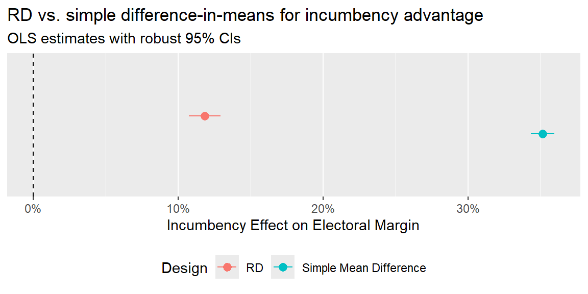
Take a look at the model summary below. The effect of incumbency is both positive and statistically significant, with a p-value well below the conventional 0.05 level. The estimate for tr indicates that incumbents got about 11.8 percentage points more votes than non-incumbents when they ran for office.
summary(rd_fit)
Call:
lm_robust(formula = y ~ tr * x, data = house, se_type = "HC1")

Standard error type:  HC1

Coefficients:
            Estimate Std. Error t value  Pr(>|t|) CI Lower CI Upper   DF
(Intercept)  0.43295   0.004327 100.058 0.000e+00  0.42447  0.44143 6554
tr           0.11823   0.005616  21.054 2.834e-95  0.10722  0.12924 6554
x            0.29691   0.016361  18.148 7.517e-72  0.26483  0.32898 6554
tr:x         0.04598   0.018043   2.548 1.085e-02  0.01061  0.08135 6554

Multiple R-squared:  0.6707 ,   Adjusted R-squared:  0.6706
F-statistic:  3892 on 3 and 6554 DF,  p-value: < 2.2e-16
This is a much more conservative estimate of the incumbency effect than you’d get by taking a naive difference in means. The below code estimates a naive model that just calculates the difference in means due to incumbency and then produces a coefficient plot summarizing the results. The naive difference in means really overshoots the size of the incumbency advantage measured with an RD design.
## estimate simple diff-in-means
lm_robust(
  y ~ tr,
  data = house,
  se_type = "HC1"
) -> smp_fit

## compare
bind_rows(
  tidy(rd_fit) |> mutate(Design = "RD"),
  tidy(smp_fit) |> mutate(Design = "Simple Mean Difference")
) |>
  filter(term == "tr") |>
  ggplot() +
  aes(estimate, term, xmin = conf.low, xmax = conf.high) +
  geom_pointrange(
    aes(color = Design),
    position = position_dodge(-.3)
  ) +
  geom_vline(
    xintercept = 0,
    lty = 2
  ) +
  labs(
    title = "RD vs. simple difference-in-means for incumbency advantage",
    subtitle = "OLS estimates with robust 95% CIs",
    x = "Incumbency Effect on Electoral Margin",
    y = NULL
  ) +
  scale_x_continuous(
    labels = scales::percent
  ) +
  scale_y_discrete(
    breaks = NULL
  ) +
  theme(
    legend.position = "bottom"
  )
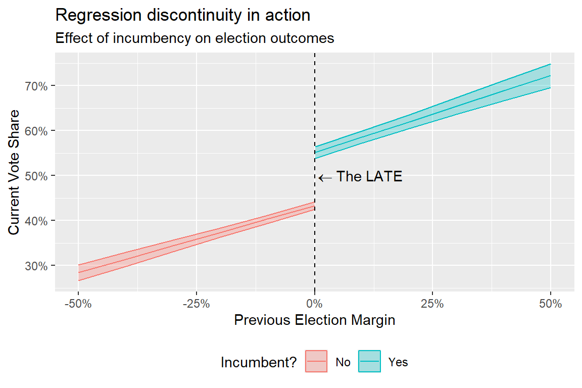
Coefficient plots are a convenient way to quickly summarize the LATE from an RD study, but a much cooler approach is to put together a plot summarizing how the predicted outcome changes conditional on the running variable. This kind of plot helps highlight the effect of the causal variable at the point of the discontinuity. The below code provides an example using the sim_pred() function I introduced in Chapter 6 on making predictions. I’ll use it to generate predicted outcomes with confidence intervals for my RD design. Once I simulate the data, I’ll summarize and plot the results. The code for the plot will give you a pretty neat and detailed graph that shows how the predicted vote share changes by the previous vote margin in a district and by incumbency status.
sim_pred <- function(model, newdata, its = 1000) {
  if(missing(newdata)) stop("The 'newdata' option is missing.")
  if(!identical(class(model), "lm_robust")) stop("The model should be a 'lm_robust' class object.")
  sim_pres <- replicate(
    n = its,
    expr = {
      nmodel <- model
      nmodel$coefficients <- MASS::mvrnorm(
        n = length(model$coefficients),
        mu = model$coefficients,
        Sigma = nmodel$vcov
      ) |> diag()
      ndata  <- newdata
      ndata$pred <- predict(nmodel, newdata = newdata)
      list(ndata)
    }
  )
  out <- dplyr::bind_rows(sim_pres)

  ## return out
  out
}

## simulate predictions
rd_fit |>
  sim_pred(
    newdata = tibble(
      x = c(seq(-.5, .5, by = 0.1), 0.001),
      tr = ifelse(x > 0, 1, 0)
    )
  ) -> sim_data

## summarize and visualize the results
sim_data |>
  group_by(x, tr) |>
  summarize(
    fit = mean(pred),
    lo = quantile(pred, 0.025),
    hi = quantile(pred, 0.975)
  ) |>
  mutate(
    tr = ifelse(tr == 1, "Yes", "No")
  ) |>
  ggplot() +
  aes(
    x = x,
    y = fit,
    color = tr,
    fill = tr
  ) +
  geom_line() +
  geom_ribbon(
    aes(ymin = lo, ymax = hi),
    alpha = 0.3
  ) +
  geom_vline(
    xintercept = 0,
    linetype = 2
  ) +
  labs(
    title = "Regression discontinuity in action",
    subtitle = "Effect of incumbency on election outcomes",
    x = "Previous Election Margin",
    y = "Current Vote Share",
    color = "Incumbent?",
    fill = "Incumbent?"
  ) +
  scale_x_continuous(
    labels = scales::percent
  ) +
  scale_y_continuous(
    labels = scales::percent
  ) +
  theme(
    legend.position = "bottom"
  ) +
  annotate(
    "text",
    x = 0,
    y = 0.5,
    label = "''%<-%'The LATE'",
    parse = T,
    hjust = 0
  )
11.4 RD’s limitations
The RD approach to causal inference is a handy tool, but it should be used responsibly. Before you start applying the RD, you need to take the local part of the LATE seriously and think carefully about bandwidth, continuity at the threshold, and fuzzy discontinuities. I talk about all these issues in more detail below.
11.4.1 Take the “local” in the LATE seriously
Underneath the RD regression estimates are a set of implied counterfactuals. Check out the below figure. As you can see, the slopes for incumbents and non-incumbents aren’t identical. Also, half of the slopes for each treatment condition are generated for sections of the running variable where no data actually exists. There are no incumbents who failed to get a positive vote margin in the previous election, and there are no non-incumbents who did. Nonetheless, the model is consistent with these potential outcomes.
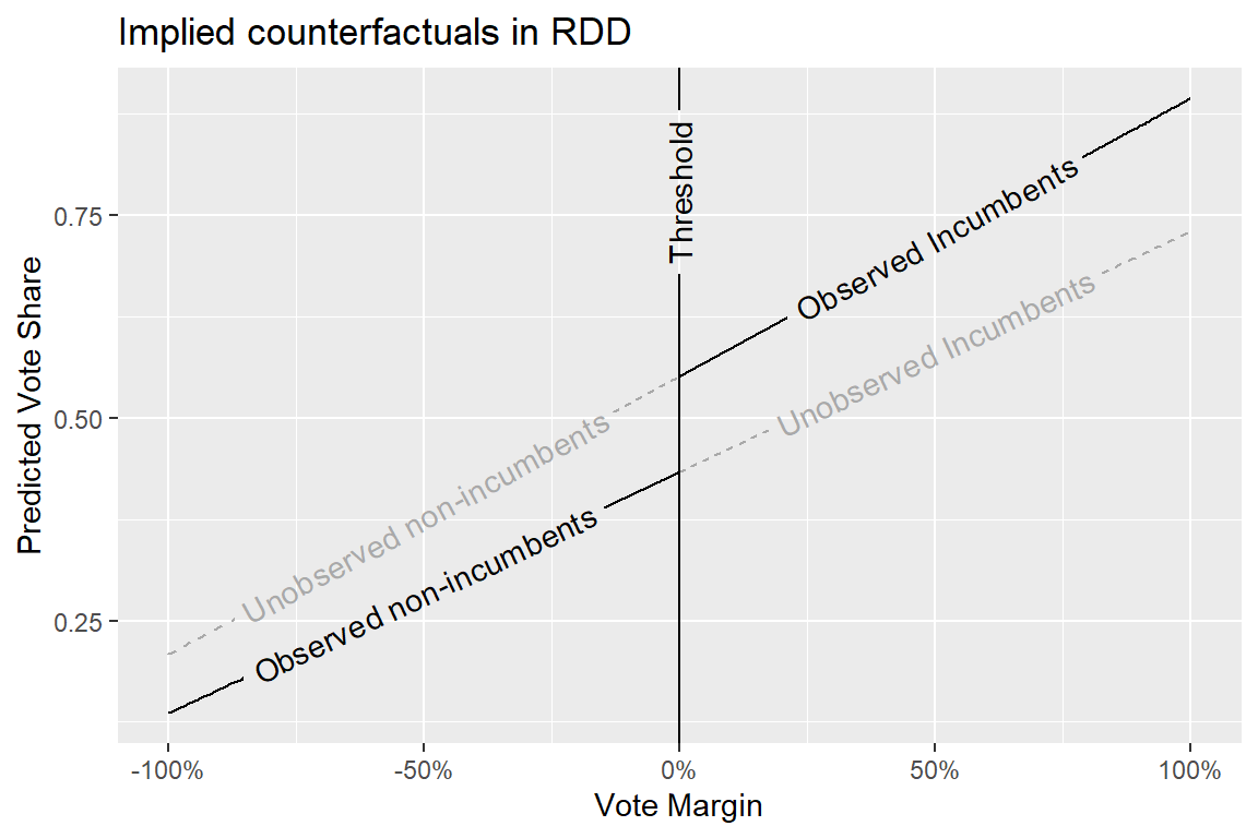
This is why it’s so critical to take the “local” part of the LATE seriously. You should avoid going beyond what the data can actually tell you, and in the case of the RD’s LATE estimate, only data points at the discontinuity exist to provide the LATE with supporting evidence. If you go even a little bit above or below the threshold, the evidence of an effect goes away, even though the model is technically consistent with effects in these places and beyond.
11.4.2 Bandwidth: Bias vs. precision
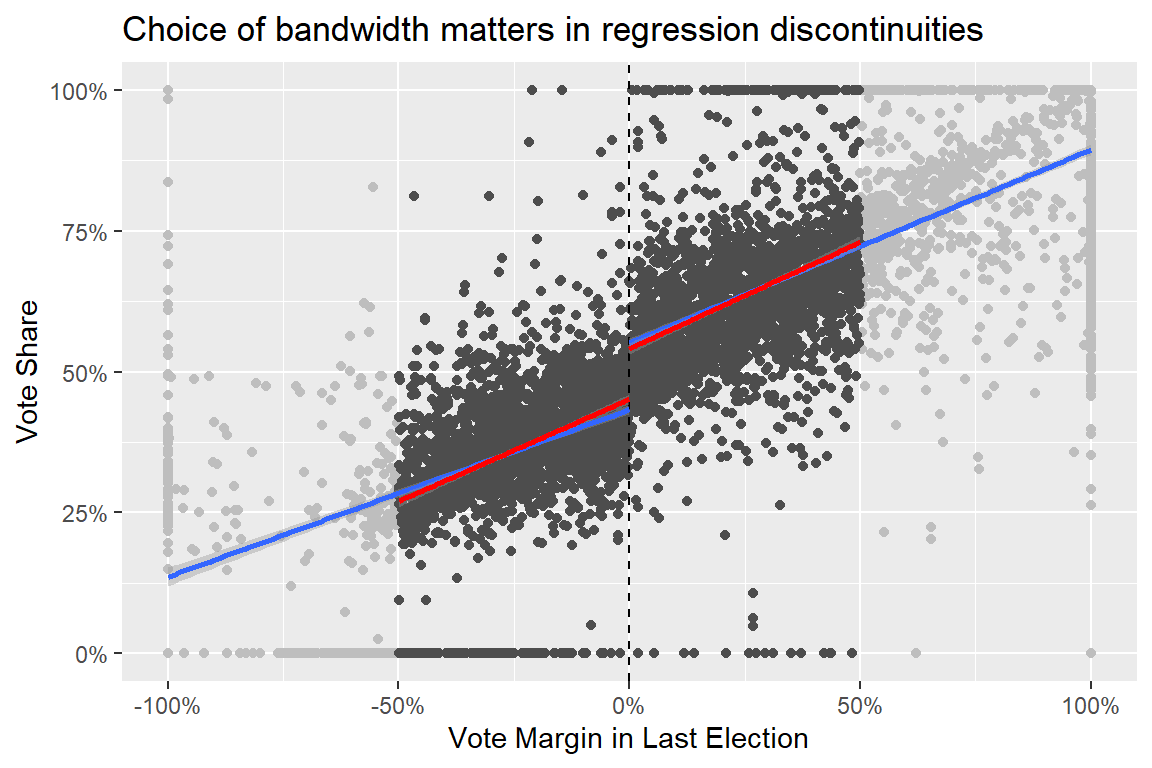
In the U.S. House incumbency data, all the data points were used, but that also means that the pre- and post-discontinuity slopes are influenced by observations that fall very far from the discontinuity. Do you really want to use information from candidates that won or lost elections by double digits to estimate the LATE for very close elections?
If you’re worried that distant observations will bias the LATE, you can control the bandwidth or binwidth of observations around the treatment threshold. This approach involves truncating your sample so that you drop observations beyond a certain distance from the discontinuity.
Say you did so with the House data by only looking at margins +/- 25 percentage points from the incumbency threshold. The code below produces a plot that overlays what the RD would look like with this bandwidth over the RD that uses all the data points. If you squint, you can see that the pre- and post-discontinuity slopes are slightly different, resulting in an equally slight decline in the magnitude of the LATE.
ggplot(house) +
  aes(x = x,
      y = y) +
  geom_point(
    color = "gray"
  ) +
  geom_point(
    data = house |> filter(between(x, -0.5, 0.5)),
    color = "gray30"
  ) +
  geom_vline(
    xintercept = 0,
    lty = 2
  ) +
  geom_smooth(
    method = lm,
    aes(group = tr)
  ) +
  geom_smooth(
    method = lm,
    data = house |> filter(between(x, -0.5, 0.5)),
    aes(group = tr),
    color = "red"
  ) +
  labs(
    x = "Vote Margin in Last Election",
    y = "Vote Share",
    title = "Choice of bandwidth matters in regression discontinuities"
  ) +
  scale_x_continuous(
    labels = scales::percent
  ) +
  scale_y_continuous(
    labels = scales::percent
  )
How much smaller is the LATE? I performed the RD design with the new bandwidth below to see, and made a coefficient plot to compare the results. The original estimate was 11.8 percentage points. The new estimate is just a bit less than 9 percentage points. And not only is the new estimate smaller, it is also statistically different from the old estimate, which you can see from the non-overlap of the confidence intervals in the coefficient plot below.
rd_fit2 <- lm_robust(
  y ~ tr * x,
  data = house |> filter(between(x, -0.5, 0.5)),
  se_type = "HC1"
)

bind_rows(
  tidy(rd_fit) |>
    mutate(Bandwidth = "None"),
  tidy(rd_fit2) |>
    mutate(Bandwidth = "+/-25 ppt")
) |>
  filter(term == "tr") |>
  ggplot() +
  aes(estimate, term, xmin = conf.low, xmax = conf.high) +
  geom_pointrange(
    aes(color = Bandwidth),
    position = position_dodge(-.3)
  ) +
  geom_vline(
    xintercept = 0,
    linetype = 2
  ) +
  labs(
    x = "Incumbency Effect",
    y = NULL,
    title = "Comparing estimation strategies",
    subtitle = "The RD estimate is more conservative with a smaller bandwidth"
  ) +
  scale_x_continuous(
    labels = scales::percent
  ) +
  scale_y_discrete(
    breaks = NULL
  ) +
  theme(
    legend.position = "bottom"
  )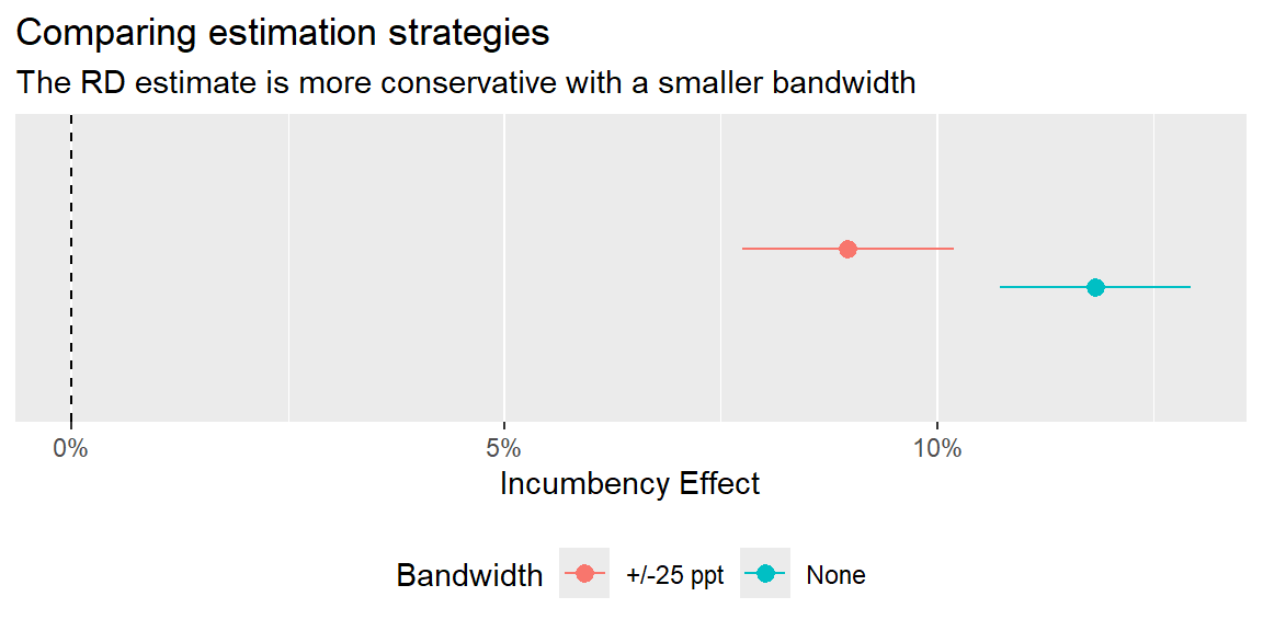
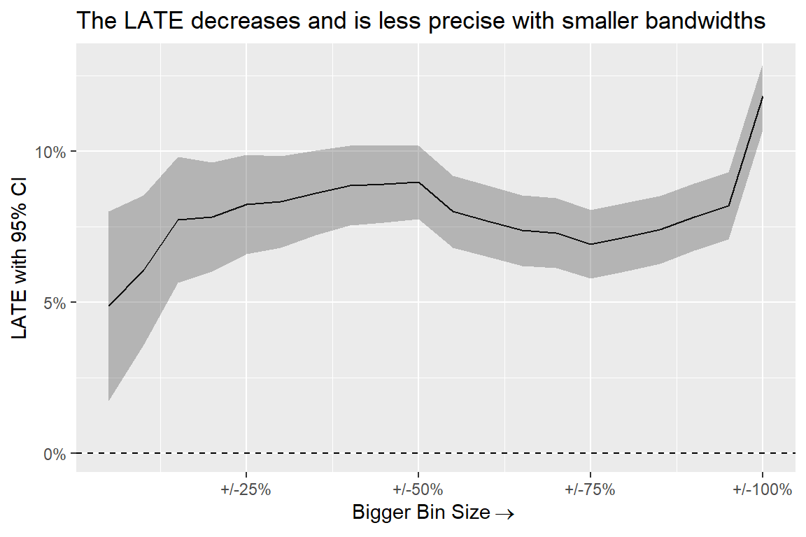
If you squint at the above results, you can see that something else changed when using a smaller bandwidth: the confidence intervals are a bit wider. Dropping data points from the analysis hurts statistical power. That means, the narrower the bandwidth, the wider the standard errors are going to get.
To better demonstrate the point, the below code iterates over a bunch of different bandwidths and then plots the estimated LATE with its 95% CI to demonstrate. As you can see, as the bandwidth gets smaller, the confidence intervals become wider while the magnitude of the LATE decreases.
# vector of bandwidths to try:
bin_sizes <- seq(0.05, 1, by = 0.05)

# estimate the RDD for each bandwidth:
bin_sizes |>
  map_dfr(
    ~ lm_robust(
        y ~ tr * x,
        data = house |>
            filter(between(x, -.x, .x)),
        se_type = "HC1"
      ) |>
      tidy() |>
      filter(term == "tr") |>
      mutate(
        bin = .x
      )
  ) -> results

# plot the results:
ggplot(results) +
  aes(x = bin,
      y = estimate,
      ymin = conf.low,
      ymax = conf.high) +
  geom_line() +
  geom_ribbon(
    alpha = 0.3
  ) +
  geom_hline(
    yintercept = 0,
    lty = 2
  ) +
  labs(
    x = expression("Bigger Bin Size"%->%""),
    y = "LATE with 95% CI",
    title = "The LATE decreases and is less precise with smaller bandwidths"
  ) +
  scale_x_continuous(
    labels = ~ paste0("+/-", 100 * .x, "%")
  ) +
  scale_y_continuous(
    labels = scales::percent
  )
This analysis provides a classic case study in the bias-variance trade-off that I introduced in Chapter 5. Recall this refers to the idea that an estimate can be a function of the truth, random background noise, and potentially some systematic error. Ideally, you want to minimize noise (reduce variance) and bias (systematic error). Unfortunately, it’s hard to minimize both at once, which is why there is a trade-off.
In this example, a smaller bandwidth removes some bias from the estimated LATE for incumbency advantage (a wider bandwidth likely yields an incumbency advantage that’s too big), but at the same time it adds variance (hence, wider confidence intervals).
There isn’t a formula that can tell you the best bandwidth that will optimally balance bias and variance. My recommendation is to be transparent and comprehensive in your analysis when using RD designs. If you aren’t sure about the best bandwidth, try out several and report the results for each one. At the very least, this lets your audience draw their own conclusions from the data.
11.4.3 Continuity at the threshold
The validity of RDs hinges on the conceit that observations at the point of the discontinuity offer apples-to-apples comparisons (that they are alike except for their exposure to the causal variable). This only works provided the discontinuity in the running variable doesn’t also influence other baseline characteristics of the units being studied that might also affect the outcome.
Take the incumbency advantage. What exactly is this capturing? Do incumbents enjoy more financing? Do they have more experience? Do voters have a status quo bias? An RD can’t tell you which factor is really the cause. Incumbency may not be the only discontinuity you need to be concerned about.
Consider another example. Say that you want to know whether funding for cities helps with public works projects and there’s a population threshold of 3,000 for getting access to these funds. You might use an RD design to see if there’s evidence that these funds are effective. But before you do, you need to make sure that this 3,000 population threshold isn’t a trigger for other changes, too. For example, maybe mayors get a bump in salary or city councils add more members once a city crosses this threshold (this happens in some countries). These factors could affect public works projects, too, making it hard to separate out the effect of funding from mayoral incentives and the political dynamics of a larger city council.
Doing a good RD design requires you to do your homework on the issue you’re studying. If there are multiple discontinuities at work, you might need to rethink your research design.
11.4.4 Fuzzy RDs
When the threshold perfectly assigns treatment, you say you have a sharp RD. But when it doesn’t, you have a fuzzy RD. In fuzzy RDs, some observations are treated just before the threshold, and/or some aren’t treated just after the threshold.
Imagine a world where third parties are more prevalent and competitive in US politics. They don’t dominate, but they’re important enough that using the 0 percentage point margin threshold for congressional data no longer offers a sharp discontinuity in incumbency status. Some candidates that got less than 50% of the vote in a previous election may still win, and thus receive the incumbency “treatment” in the next election. You can simulate this by randomizing some observations below the 0 percentage point margin threshold to receive incumbency status:
house |>
  group_split(
    between(x, -0.1, 0)
  ) -> fuzzy_house
fuzzy_house[[2]]$tr <- sample(0:1, length(fuzzy_house[[2]]$tr), T)
fuzzy_house <- bind_rows(fuzzy_house)
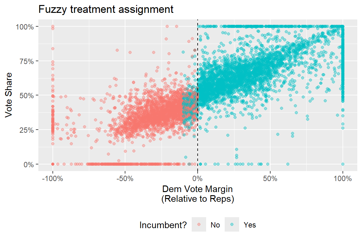
Now, if you plot a candidate’s vote share by previous vote margin, you can clearly see that treatment is no longer perfectly determined by the running variable. Check out the results below. Some candidates that got less than 50% of the vote in a previous election won and are now incumbents.
ggplot(fuzzy_house) +
  aes(x = x,
      y = y,
      color = ifelse(tr==1, "Yes", "No")) +
  geom_point(
    alpha = 0.4
  ) +
  geom_vline(
    xintercept = 0,
    lty = 2
  ) +
  labs(
    x = "Dem Vote Margin\n(Relative to Reps)",
    y = "Vote Share",
    color = "Incumbent?",
    title = "Fuzzy treatment assignment"
  ) +
  scale_x_continuous(
    labels = scales::percent
  ) +
  scale_y_continuous(
    labels = scales::percent
  ) +
  theme(
    legend.position = "bottom"
  )
To recover an estimate of the LATE when things are fuzzy, you need to use an instrumental variables (IV) approach, where you estimate two regression models in succession. In the first-stage regression, the treatment (incumbency) is predicted by a model that includes the running variable (previous election margin) and an indicator for the discontinuity threshold (winning 50% or more of the vote), and their interaction. Then, in the second-stage regression, the main outcome is predicted by a model that includes the predicted treatment from the first-stage regression, the running variable, and their interaction. The estimate in the second-stage regression should remove the bias that comes from fuzzy treatment assignment by using only variation in the treatment predicted by crossing the running variable threshold.
An IV regression can be done in R using {estimatr}’s iv_robust() function. It estimates a model where being before or after the threshold is used as an instrument for being an incumbent. In this hypothetical example, treating the discontinuity as a sharp cut-off for incumbency under-estimates the incumbency advantage, accounting for the fuzziness of incumbency assignment yields a larger estimate.
## Use iv_robust
fuzzy_fit <- iv_robust(
  y ~ tr * x | (x > 0) * x,
  data = fuzzy_house
)

## Check with "naive" sharp RD
sharp_fit <- lm_robust(
  y ~ tr * x,
  data = fuzzy_house
)

## Compare
bind_rows(
  tidy(sharp_fit) |>
    mutate(RD = "Sharp"),
  tidy(fuzzy_fit) |>
    mutate(RD = "Fuzzy")
) |>
  filter(term == "tr") |>
  ggplot() +
  aes(estimate, term, xmin = conf.low, xmax = conf.high) +
  geom_pointrange(
    aes(color = RD),
    position = position_dodge(-.3)
  ) +
  geom_vline(
    xintercept = 0,
    linetype = 2
  ) +
  labs(
    x = "Incumbency Effect",
    y = NULL,
    title = "Comparing estimation strategies",
    subtitle = "The Sharp vs. Fuzzy RD Design"
  ) +
  scale_x_continuous(
    labels = scales::percent
  ) +
  scale_y_discrete(
    breaks = NULL
  ) +
  theme(
    legend.position = "bottom"
  )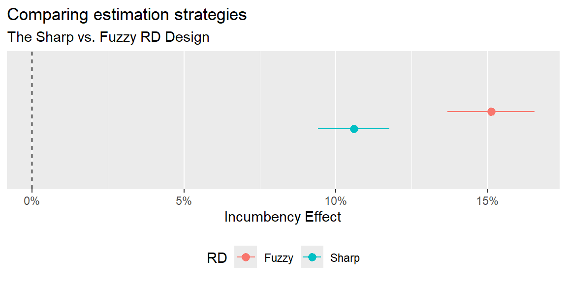
Importantly, the fuzzy RD estimate isn’t actually better in this example because I assigned some observations to the treatment condition that in actuality weren’t treated. Take the results from this analysis as a serious attempt to handle a situation with fuzzy treatment assignment, rather than as a literal estimate of the effect of incumbency.
11.5 Conclusion
RDs are a great tool for causal inference, and they have many advantages over the SOO design. To make them work, you need a running variable that defines a threshold for a discontinuity in treatment assignment. Because this threshold is often arbitrary, you can act as though treatment assignment at the threshold is random and estimate a local average treatment effect (LATE) at the point of the discontinuity.
Be warned that nature or public policy-makers don’t always use arbitrary thresholds, so that limits when you can use this kind of design. Even when you can, remember that the causal effect you get from this approach is local to the point of the discontinuity, which limits your ability to make sweeping generalizations about causal effects. In exchange for getting better causal identification with the RD compared to the SOO, your claims must inevitably become more narrow.
RD designs also require tough judgment calls, and you need to make sure you fully understand the process that led to treatment assignment. You need to consider the size of the bandwidth before and after the threshold for treatment assignment. A larger bandwidth will give you more precision, but a smaller bandwidth will remove bias. You also need to check whether factors other than your causal variable of interest change at the threshold for treatment assignment as well. If too many things change at once at a threshold, this threatens your ability to draw clean causal inferences. Finally, you may run into scenarios where treatment assignment is fuzzy. Some observations that fall short of a threshold may still get treatment, and others that cross the threshold may not. You need to make adjustments if this happens.
The next research design I’ll talk about is very similar to RD, but it can be applied to contexts where a running variable isn’t available. It’s called a difference-in-differences design.