# this is a comment that won't run any code
1 + 3 # this is some code that will run (but this comment won't)
[1] 4# 1 + 3Learning objectives:
R and RStudio are great tools for data visualization and analysis. They are great both because they are open source (meaning you can use them for free) and because they are used by a large community of scientists, researchers, and analysts who, over the years, have developed and maintained a vast ecosystem of R packages that offer specialized tools for dealing with nearly any kind of problem you can imagine.
I should warn you that there are tradeoffs in exchange for these benefits. The R programming language has a steep learning curve (and it will be steeper for some than for others), and it takes time to orient yourself to RStudio. For these reasons, before we get to the technical details of data visualization, we need to become familiar with the basics of R and RStudio.
First things first, you need to be able to access the software. For those taking DPR 101, you can do so via Denison’s R server at r.denison.edu by logging-in with your Denison credentials. If you’re off campus, you’ll need a VPN connection to access the server. You can read more about how to do that via one of the following links:
Once you access the server, you may already be in a project space. If not, you’ll need to start a new session.
You aren’t limited to only using the Denison server. If you’d rather install the relevant software on your computer, you’re free to do so. You can learn more about how to download R and RStudio for your desktop at https://posit.co/download/rstudio-desktop/.
If you already have R and RStudio, that’s great! You’re already good to go.
Once you’ve accessed the software (whether on the server or on your own desktop) the RStudio environment you see before you should have a few different components, including:
At this point you should be able to tell that a lot is going on in RStudio. There’s a reason why RStudio is called an “integrated development environment” (IDE). It is a language-agnostic application separate from R itself. Within it, you can work with many different languages (not just R, but Python as well). Having an IDE to help you interface with R is an amazing resource, because R proper is pretty spartan all on its own, and it definitely falls short as far as user-friendly software goes. RStudio lets you organize files, save your work in projects, and write reports all within a single environment. You many not appreciate how big of a deal this is, but for those of us who started working with R without the aid of an IDE, the difference this makes feels like the equivalent of switching to using a scientific calculator after years of using an abacus.
The best way to work in RStudio is to save your work in projects. This lets you organize all your work in a tidy way, and it also ensures that the locations of files (like datasets) you want to use are easily accessible with minimal lines of code.
If you look at the upper right corner, you can see a cube with an “R” in it. If you select that you’ll see a drop-down menu. Select “New Project” -> “New Directory” -> “New Project” -> enter a new directory name for your project -> use “browse” to find a place in your files you’d like to save your work then -> “create.” For this class, I recommend creating a project called “DPR 101” that way it’s obvious to your future self that this is where your work for this class is located.
After you create your project, I recommend creating two different folders. Call one _data and the other _code. Any datasets that you need to download for this class you can save in the _data folder, and all the Quarto files you use for note-taking and assignments can go in the _code folder.
I’ve been teaching long enough already to know that most of you have bad file hygiene, and many of you will probably ignore my recommended filing system. Sooner or later, you’ll need to clean up your act, so why not start now? It’ll go a long way in helping you avoid errors down the road.
There are many kinds of files that you can work in within RStudio. The one that we’ll use in this class is called a Quarto file (.qmd).
Quarto documents are a great place to:
You can also use these documents to write reports, presentation slides, or even websites. This very book was created using Quarto files.
These features of working in Quarto are great for learning to code. You can make notes to yourself in plain text about what data you’re working with and what your code is supposed to be doing. There are lots of helpful resources out there for working with Quarto, too. I recommend starting with the main Quarto page. There’s also a set of chapters dealing with Quarto documents in R for Data Science (2e) which you can access at https://r4ds.hadley.nz/quarto.
When you work with Quarto, you can either work in the source version of the document, or the visual version. The latter is a visual editor of a Quarto document that makes it really easy and intuitive to create section headers, use different font faces, and drop in code chunks. It’s up to you which way you want to go. Some people like the no-frills source editor (it’s also slightly less “buggy”), but a pro with the visual editor is that it’s a little more like working with a Word document in that you can easily adjust the font face, drop in section headers in such a way that they actually look like headers, etc. What’s really nice, no matter which editor you choose, is that you can toggle back and forth between them with one click. If you look at the top left corner of the Quarto document you’re working in, you will see just down from the blue save icon and just right of the Bold text icon buttons that say “Source” and “Visual.” Just click on the view you want.
Quarto files aren’t just useful for writing and running code and making notes. You can convert your document into a report by using the “Render” button at the top center of the Quarto file (it has the big blue arrow next to it).
When you render a Quarto document, you can update a few things about how it renders in the YAML. This is the bit of code that appears at the very tip top of your quarto document, and the acronym stands for “yet another markup language.” This is a block of human-readable code that describes how to configure a file.
Here’s a good summary of the options you have for updating the YAML.
When you use Quarto, your notes/comments/writing in plain text will be interspersed with R code bocks.
An R code block is created using three backticks (“```”) followed by an “r” in brackets, and then it’s closed with three more backticks.
Think of each code block as a self-contained space for writing and running a specific bit of code. After you make a code block and write some code in it, you have a bunch of different options for running it.
In addition to making notes in plain text around your code blocks, you can make notes inside code blocks as well. Anything that follows a # in a bit of R code is “commented out.” That means R knows not to run anything that follows the hashtag in the code. For example:
# this is a comment that won't run any code
1 + 3 # this is some code that will run (but this comment won't)[1] 4# 1 + 3You also can use a hashtag-vertical line combo (#|) to give specific preferences for how a given code block runs. Say you don’t want a particular code block to appear in a rendered document. You would write the following message indicating echo is “false” followed by the code you want to run.
#| echo: false
2 + 2
If you’re writing code to make a data visualization, you can add an option to include a figure caption (which will appear below the data visual when you render your document) and you can control the data visualizations dimensions. Here’s a very simple example using the plot() function:
#| fig-cap: "An example figure with a label"
#| fig-height: 4
#| fig-width: 6

plot(mtcars$wt, mtcars$mpg)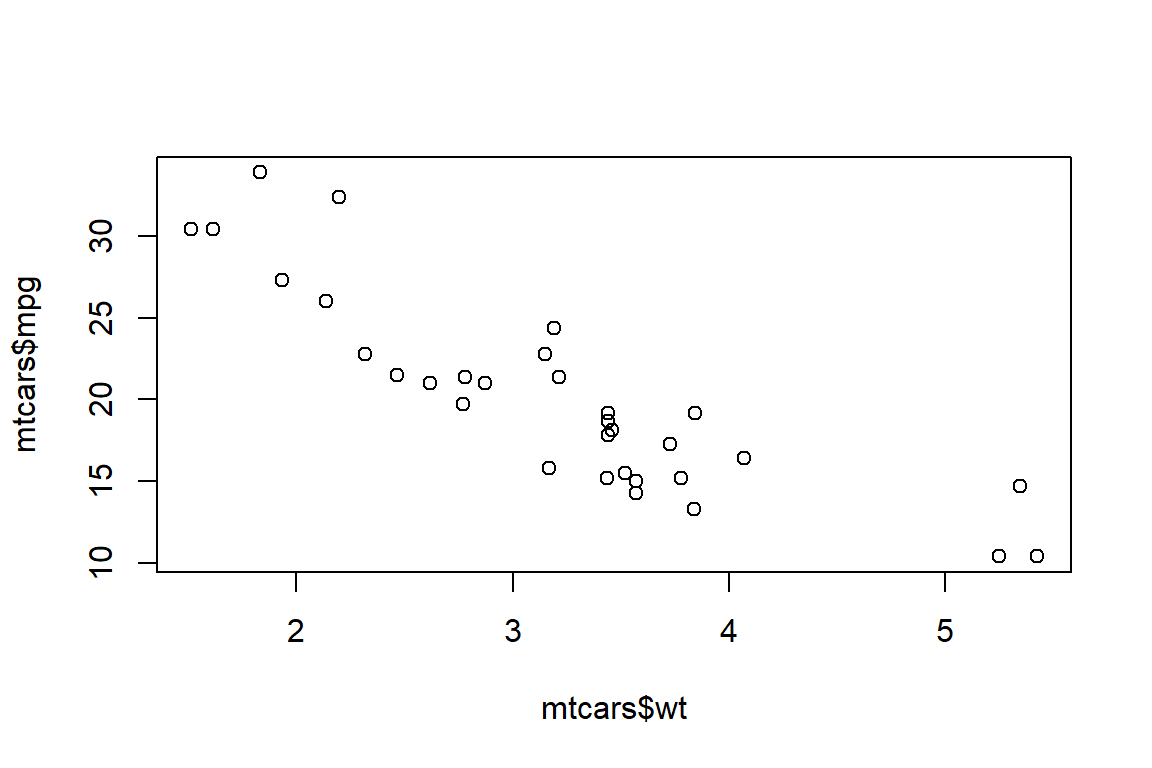
There are a few things you need to know about R. First and foremost, R is not just software, it’s a language. Just like learning any language, fluency in R takes time and a lot of practice.
R specifically is an “object oriented” and “functional” programming language. That means a few things.
First, everything in R has a name. You refer to the names of things to examine them or use them. These things can be variables or datasets that you manipulate, or functions that you use to perform operations.
Like any language, there are some grammatical rules in R that you should never break (and cannot break if you tried). For example, words like TRUE or FALSE, Inf or else, and several others have been reserved for core programming purposes and you couldn’t name something in R one of these things if you tried.
Other words or letters, like q, c, or mean can technically be used to refer to other things, but do so at your own peril! These are the names of basic functions in R, and if you give other things in R the same names, R will get confused and angry with you.
R is also case sensitive. So if something is named This R won’t know what you’re talking about if you try to call This by instead writing this.
Second, everything in R is an object.
Say we use the command c(), which is a function that stands for “concatenate.” It takes a sequence of values and returns a vector where each element is accessible:
c(1, 2, 4, 8, 16, 32)[1] 1 2 4 8 16 32The output from the above is just all the elements in the vector we created using c(). If we didn’t want this to just appear in the console but instead have it saved, we need to assign the vector a name, which then saves it as an object:
my_numbers <- c(1, 2, 4, 16, 32)Now, every time we call the object my_numbers, the output will appear in the console (or as the output of a code block):
my_numbers[1] 1 2 4 16 32Each of the numbers in this vector can be accessed directly, too. This is done using square brackets [] after the name of the object. The below code pulls out the thrid element in the vector called my_numbers:
my_numbers[3][1] 4We created my_numbers using an assignment operator <-. When you want to save something as an object, you need to use an assignment operator, which (by the way) can work not only from the right to the left (the usual way), but also from the left to the right. The latter way is sometimes called “reverse assignment,” but I this is a bit of a misnomer because I think assigning things left to right makes more sense (as an English speaker). Here’s an example using both:
# normal assignment
x <- c(1, 2, 3)

# reverse assignment
c(4, 5, 6) -> y
You can technically use the = operator to assign things, too, but there are some pitfalls to note about this approach:
Generally, it’s considered bad grammar in R to use = for assignment. Instead, we use = inside of functions (coming up next) to set commands or feed objects to functions when we want to perform an operation.
Speaking of functions, just about everything you do in R with be with a function. A function is a special kind of object that performs actions for you. You feed it an input (like an object) and it provides an output (which you can assign to a new object for later use). A good way to think about functions is that they’re verbs that let you do things with different objects.
For example, there’s a function called mean() which we can use on the object my_numbers:
mean(x = my_numbers)[1] 11The function does exactly what its name suggests—it returns the mean or average of whatever numerical vector you feed it.
When using some functions you don’t always have to be so explicit about the inputs you give them. Many functions expect inputs to be given in a certain order. mean() for example expects the first input to be the vector you want to take the mean of. Because of this, to take the mean of my_numbers you could just write:
mean(my_numbers)[1] 11In the long-run, knowing little short-cuts like this saves you from having to be so verbose in your code.
Like all functions, mean() has some rules about what kinds of inputs it will accept. If you feed it nothing, it’ll give you an error that says Error in mean.default() : argument "x" is missing, with no default. In short, a function can’t do something to nothing. Also, if you feed it non-numerical data, it’ll give you a warning and return NA:
my_words <- c("Hello", "World!")
mean(x = my_words)
Warning in mean.default(x = my_words): argument is not numeric or logical:
returning NA[1] NAWhat’s the average of “Hello” and “World!”? I dunno, and neither does R. You can’t use mean() to compute a mean for an object that doesn’t have numerical value.
Now you may be asking yourself, “how am I supposed to remember all the rules for how to use every function I may ever need to use!?” Mercifully, if you ever want to learn more about a function, you can ask R to show you its help file. All you need to do is write something like help(function_name) in the console. You could just write ?function_name in the console as well. For example, go to the console and write ?mean, hit enter/return and see what happens. You’ll see the help file pop up over in the lower right quadrant of your work space under the “Help” tab.
On the subject of functions, we should talk about the fact that they come in packages. Some functions, like mean(), are in the base R package which is already open and ready to go the moment you open R. Other functions can’t be used until you attach the package that a function lives in using the library() function.
In this class, we’ll use the R package called {tidyverse} in every session (note that we use the notation {} and the package name inside to signify that we’re talking about a package). The {tidyverse} is actually a package of packages that have functions that are meant to be used together. Rather than attach each package in the tidyverse individually, if we write library(tidyverse) all these packages and the functions they contain are immediately accessible to us.
library(tidyverse)Warning: package 'tidyverse' was built under R version 4.2.3Warning: package 'ggplot2' was built under R version 4.2.3Warning: package 'tibble' was built under R version 4.2.3Warning: package 'tidyr' was built under R version 4.2.3Warning: package 'readr' was built under R version 4.2.3Warning: package 'purrr' was built under R version 4.2.3Warning: package 'dplyr' was built under R version 4.2.3Warning: package 'stringr' was built under R version 4.2.3Warning: package 'forcats' was built under R version 4.2.3Warning: package 'lubridate' was built under R version 4.2.3── Attaching core tidyverse packages ──────────────────────── tidyverse 2.0.0 ──
✔ dplyr 1.1.2 ✔ readr 2.1.4
✔ forcats 1.0.0 ✔ stringr 1.5.0
✔ ggplot2 3.5.0 ✔ tibble 3.2.1
✔ lubridate 1.9.3 ✔ tidyr 1.3.0
✔ purrr 1.0.2
── Conflicts ────────────────────────────────────────── tidyverse_conflicts() ──
✖ dplyr::filter() masks stats::filter()
✖ dplyr::lag() masks stats::lag()
ℹ Use the conflicted package (<http://conflicted.r-lib.org/>) to force all conflicts to become errorsSome packages have already been pre-installed for you if you’re using the Denison server. If you aren’t, you’ll need to install these using the install.packages() function. Now, beware that this function for installing packages only works for packages that have been made available on R’s CRAN (Comprehensive R Archive Network). Many packages not on the CRAN have been published to an open source repository on GitHub, and to install these packages you’ll need to use slightly different syntax.
One example of such a package is {coolorrr}, which is a package that I personally created to make working with color palettes in figures easier. To install it, you’ll need to run the following in your console:
devtools::install_github("milesdwilliams15/coolorrr")Notice in the above that I used double colons :: after devtools. If you ever only want to access a single function from a package ({devtools} is a package that helps with installing packages from sources like GitHub), but don’t want to attach the full package in R, you can write the package name followed by :: to call the function you want. The syntax will be something like package_name::function_name().
R is many things, including a glorified calculator. You can use a lot of different operations like * for multiplication, / for division, + for addition, and - for subtraction.
R also uses a number of logical operators like AND &, OR |, NOT !, EQUAL TO ==, GREATER THAN >, GREATER THAN OR EQUAL TO >=, LESS THAN <, LESS THAN OR EQUAL TO <=, NOT EQUAL TO !=, and IN %in%.
Remember the x and y objects I created earlier? Let’s try out some of these operations on them and see what happens:
# Mathematical operations
x + y # addition
[1] 5 7 9x - y # subtraction[1] -3 -3 -3x * y # multiplication[1] 4 10 18x / y # division[1] 0.25 0.40 0.50# Logical operations
x == y # equivalence[1] FALSE FALSE FALSEx <= y # x less than or equal to y?[1] TRUE TRUE TRUEx %in% y # are x values in y?[1] FALSE FALSE FALSENotice that mathematical operators return numerical outputs, while logical operators return logical outputs (TRUE or FALSE). While distinct, R will treat logical values as 0 (FALSE) or 1 (TRUE) under certain conditions. For example, you can take the mean of a vector of TRUE and FALSE values you get just the same value as if you had given the function a set of 0s and 1s:
mean(x = c(0, 1))[1] 0.5mean(x = c(F, T)) # these are the same[1] 0.5As a shortcut, you can just write T for TRUE and F for false, as I did in the above block, and R will know what you mean.
Another feature of R (at least for more recent versions) is the base R “pipe” operator |>. This operator lets you tell R you want to give some object to a particular function, like so:
x |>
  mean()
[1] 2This might seem unnecessary, but this ability to pipe from one object to some function comes in handy when you want to perform many different sets of operations in succession.
The idea of piping isn’t new to R. In fact, this ability has existed for some time in the form of a different pipe operator that looks like this: %>%. This operator is available in the {magrittr} package which is also opened once you open the {tidyverse}. Both the |> and %>% operators work very similarly but they abide by slightly different rules. You can read more about the differences by reading this article written by the folks responsible for {tidyverse}. The TL;DR version of it is that |> is computationally faster and a good general use tool while %>% is computationally slower but will be better to use in some specialized circumstances. Occasionally in the code that appears in this book you’ll see me use one or the other pipe depending on the circumstance.
All of the work we do in this class will involve datasets. Think of these as tables that store data in a central location for ease of access and use.
mtcars is a dataset that already comes pre-installed in R. Let’s poke around it a bit to get a sense for what we can do with datasets. We can check out the first 10 rows of the data using the head() function:
head(mtcars, 10) mpg cyl disp hp drat wt qsec vs am gear carb
Mazda RX4 21.0 6 160.0 110 3.90 2.620 16.46 0 1 4 4
Mazda RX4 Wag 21.0 6 160.0 110 3.90 2.875 17.02 0 1 4 4
Datsun 710 22.8 4 108.0 93 3.85 2.320 18.61 1 1 4 1
Hornet 4 Drive 21.4 6 258.0 110 3.08 3.215 19.44 1 0 3 1
Hornet Sportabout 18.7 8 360.0 175 3.15 3.440 17.02 0 0 3 2
Valiant 18.1 6 225.0 105 2.76 3.460 20.22 1 0 3 1
Duster 360 14.3 8 360.0 245 3.21 3.570 15.84 0 0 3 4
Merc 240D 24.4 4 146.7 62 3.69 3.190 20.00 1 0 4 2
Merc 230 22.8 4 140.8 95 3.92 3.150 22.90 1 0 4 2
Merc 280 19.2 6 167.6 123 3.92 3.440 18.30 1 0 4 4This dataset is a class of object in R called a “dataframe.” R objects have different classes (classifications), by the way.
To access a single column of a dataframe, just use the syntax dataset$variable:
mtcars$mpg [1] 21.0 21.0 22.8 21.4 18.7 18.1 14.3 24.4 22.8 19.2 17.8 16.4 17.3 15.2 10.4
[16] 10.4 14.7 32.4 30.4 33.9 21.5 15.5 15.2 13.3 19.2 27.3 26.0 30.4 15.8 19.7
[31] 15.0 21.4A particularly useful way to save a dataframe in R is as a tibble. To convert a dataframe to a tibble (which is a special kind of dataframe) just write:
mtcars_tb <- as_tibble(mtcars)
head(mtcars_tb, 10)
# A tibble: 10 × 11
mpg cyl disp hp drat wt qsec vs am gear carb
<dbl> <dbl> <dbl> <dbl> <dbl> <dbl> <dbl> <dbl> <dbl> <dbl> <dbl>
1 21 6 160 110 3.9 2.62 16.5 0 1 4 4
2 21 6 160 110 3.9 2.88 17.0 0 1 4 4
3 22.8 4 108 93 3.85 2.32 18.6 1 1 4 1
4 21.4 6 258 110 3.08 3.22 19.4 1 0 3 1
5 18.7 8 360 175 3.15 3.44 17.0 0 0 3 2
6 18.1 6 225 105 2.76 3.46 20.2 1 0 3 1
7 14.3 8 360 245 3.21 3.57 15.8 0 0 3 4
8 24.4 4 147. 62 3.69 3.19 20 1 0 4 2
9 22.8 4 141. 95 3.92 3.15 22.9 1 0 4 2
10 19.2 6 168. 123 3.92 3.44 18.3 1 0 4 4There are lots of ways for peering into a dataset to get a sense for its structure (what it contains, how big it is, etc.). For example, you can use summary() to get some quick summary statistics that tell you about the variables in a dataset:
summary(mtcars_tb) mpg cyl disp hp
Min. :10.40 Min. :4.000 Min. : 71.1 Min. : 52.0
1st Qu.:15.43 1st Qu.:4.000 1st Qu.:120.8 1st Qu.: 96.5
Median :19.20 Median :6.000 Median :196.3 Median :123.0
Mean :20.09 Mean :6.188 Mean :230.7 Mean :146.7
3rd Qu.:22.80 3rd Qu.:8.000 3rd Qu.:326.0 3rd Qu.:180.0
Max. :33.90 Max. :8.000 Max. :472.0 Max. :335.0
drat wt qsec vs
Min. :2.760 Min. :1.513 Min. :14.50 Min. :0.0000
1st Qu.:3.080 1st Qu.:2.581 1st Qu.:16.89 1st Qu.:0.0000
Median :3.695 Median :3.325 Median :17.71 Median :0.0000
Mean :3.597 Mean :3.217 Mean :17.85 Mean :0.4375
3rd Qu.:3.920 3rd Qu.:3.610 3rd Qu.:18.90 3rd Qu.:1.0000
Max. :4.930 Max. :5.424 Max. :22.90 Max. :1.0000
am gear carb
Min. :0.0000 Min. :3.000 Min. :1.000
1st Qu.:0.0000 1st Qu.:3.000 1st Qu.:2.000
Median :0.0000 Median :4.000 Median :2.000
Mean :0.4062 Mean :3.688 Mean :2.812
3rd Qu.:1.0000 3rd Qu.:4.000 3rd Qu.:4.000
Max. :1.0000 Max. :5.000 Max. :8.000 You can use the glimpse() function to check the data’s structure:
glimpse(mtcars_tb)Rows: 32
Columns: 11
$ mpg <dbl> 21.0, 21.0, 22.8, 21.4, 18.7, 18.1, 14.3, 24.4, 22.8, 19.2, 17.8,…
$ cyl <dbl> 6, 6, 4, 6, 8, 6, 8, 4, 4, 6, 6, 8, 8, 8, 8, 8, 8, 4, 4, 4, 4, 8,…
$ disp <dbl> 160.0, 160.0, 108.0, 258.0, 360.0, 225.0, 360.0, 146.7, 140.8, 16…
$ hp <dbl> 110, 110, 93, 110, 175, 105, 245, 62, 95, 123, 123, 180, 180, 180…
$ drat <dbl> 3.90, 3.90, 3.85, 3.08, 3.15, 2.76, 3.21, 3.69, 3.92, 3.92, 3.92,…
$ wt <dbl> 2.620, 2.875, 2.320, 3.215, 3.440, 3.460, 3.570, 3.190, 3.150, 3.…
$ qsec <dbl> 16.46, 17.02, 18.61, 19.44, 17.02, 20.22, 15.84, 20.00, 22.90, 18…
$ vs <dbl> 0, 0, 1, 1, 0, 1, 0, 1, 1, 1, 1, 0, 0, 0, 0, 0, 0, 1, 1, 1, 1, 0,…
$ am <dbl> 1, 1, 1, 0, 0, 0, 0, 0, 0, 0, 0, 0, 0, 0, 0, 0, 0, 1, 1, 1, 0, 0,…
$ gear <dbl> 4, 4, 4, 3, 3, 3, 3, 4, 4, 4, 4, 3, 3, 3, 3, 3, 3, 4, 4, 4, 3, 3,…
$ carb <dbl> 4, 4, 1, 1, 2, 1, 4, 2, 2, 4, 4, 3, 3, 3, 4, 4, 4, 1, 2, 1, 1, 2,…Every time you’re done working, make sure you do a few things:
You should always perform the above three steps when you close out (with special emphasis placed on step 2). This ensures R is always running smoothly and efficiently.
Be patient with yourself as you start working in R and RStudio. At the same time that you are familiarizing yourself with new software, you also are learning to speak a new language. If things don’t make sense at first, that’s okay. That’s normal.
I can’t possibly anticipate every possible issue you may run into as you use R, but I can give you a heads up about some common mistakes people make:
> at the bottom of the console, all is good. If you see a + then something only partially ran.x, then ran a function on it and saved the output as x, then tried to go back and run an old chunk on x only to find that it spits out an error. The old x that used to work with a function now no longer does because the new x isn’t the same thing!If you’re overwhelmed by all of this, I don’t blame you. But just like it’s a bad idea to build a house on sand, it’s a bad idea to jump into data analysis in R without first laying a solid foundation. If you need to, read and re-read parts of these notes before you jump into the next chapter. And after you move on, don’t forget that you can always come back to this chapter for reference.
Alright, without all of that out of the way, let’s move to Part II of the book dealing with descriptive data analysis.