library(tidyverse)7 Data Wrangling
7.1 Goals
- Understand the importance of data wrangling.
- Apply the main
{dplyr}functions to mutate and summarize a dataset. - Layer complexity by chaining together multiple
{dplyr}functions. - Use
{tidyr}functions to reshape datasets.
7.2 Introduction
In this second part of data visualization for political research, we’re going to delve into an ongoing debate about the so-called long peace. This term is used by some to describe a pattern of declining armed conflict (generally speaking) since the mid-twentieth century. While international and civil conflicts have certainly erupted during this period, and continue to, proponents of the long peace argue that truly deadly, systemic wars like World War I and World II haven’t occurred and are unlikely to in the future. Some go further and argue that wars in general are becoming less frequent and are less deadly when they happen. Many have used data to back up this claim (Steven Pinker is a great example).
Not everyone agrees with this idea. I think one of the best arguments against the long peace is made by the political scientist Bear Braumoeller who uses some high quality data and specialized statistics to show that evidence of the long peace is weak, if nonexistent. Other researchers using similar data draw the same conclusion.
Ultimately, the long peace remains an unsettled issue. Questions about data quality and measurement are partly to blame. Depending on how you slice and dice a particular dataset, the trend in war occurrence and deadliness can look positive, negative, or constant. And the trouble is, many of these competing ways of showing the data are perfectly justifiable.
In this and the coming chapters, we’ll spend some time exploring data on international conflict to see what we can say about long-term trends in war. If the long peace holds any water, we should expect to see two things in our data. The first is that the rate of conflict onset (that’s a measure of whether a new war has started) should be declining over time. The second is that the severity of conflict (a measure of how many people died as a direct result of fighting) should be declining over time as well.
As will become quickly apparent, we’ll have to make a lot of choices about how to handle and show the data. Some of these choices, while seemingly trivial, can add up to big differences in what the data tell us about trends in war.
We’ll also get some experience with techniques for showing trends in data over time. Some ways of presenting trends are more useful than others, and there are some common pitfalls that we’ll talk about and try to avoid.
But, before we get to data visualization, I want to spend some time talking about data wrangling, which is an essential step in data visualization. Often times the data we want to use is not in the format we’d like it to be, so it is essential that we know how to use different tools for reshaping our data to prep it for analysis and visualization. Let’s get to it.
7.3 The importance of data wrangling
Data wrangling is the process of cleaning and reshaping a dataset to make it ready for data visualization or analysis. Many of the datasets you’ve used up to now have required only minimal data wrangling, but in many real-world settings you won’t be so lucky. You therefore need to know how to clean, collapse, and reshape data so you can use it to generate insights.
The {tidyverse} approach to statistical programming in R provides a number of helpful tools or “verbs” for performing data wrangling. We’ll walk through these verbs below and how to use them. While you probably won’t master them over night, with time and practice these tools will become easier to use.
7.4 Using {dplyr} for data mutation and summaries
The {dplyr} package is a powerful tool for letting us transform data into what we need for analysis and data visualization. This package is part of the {tidyverse} and is automatically opened when you use library(tidyverse).
There are 6 key {dplyr} functions that you need to know about:
filter(): Choose observations based on their values using Boolean operators (==,!=,>,<,>=,<=)arrange(): Reorder the rows of a dataset based on the values of a variableselect(): Choose variables (columns) based on their namesmutate(): Create new variables or modify existing onessummarize(): Collapse many variables into a single summary or a summary by certain categoriesgroup_by(): Specify the scope of the function that you want to perform (for example, calculate the average votes cast for a candidate by education level).
We’ll start by opening the tidyverse as always:
While the functions available with {dplyr} are functions, sometimes we call them “verbs” because we use them to do certain operations with our data. Moreover, a nice feature of working with these verbs is that we can chain them together to perform a succession of possibly highly complex data transformations. We can chain together multiple {dplyr} “layers” like with ggplot using the |> pipe operator. We’ve already seen this in action in some previous code.
A quick note on the pipe: Once upon a time we used %>% for pipes. You can still use this version of the pipe, but the most up-to-date version of R provides |> as a new alternative. There are just a few minor differences in how they work, but these differences usually don’t matter. A nice feature of |> is that it is computationally faster than %>% (in addition to being slightly quicker to write). If you have a lot of code to run and lots of computations to deal with, any small efficiency gain is a win.
Back to using {dplyr} verbs… Here’s how the workflow with these verbs generally works:
- First, we start with a data object.
- Then, we add verbs that describe what to do with the data using column (variable) names and other instructions. Note that we don’t need to put the column names in quotes. Because we’ve already specified the data object that they are contained in, R will be able to find them as a “known” object.
- The output is a new data frame, which we can save as a new object.
For example, say we wanted to create a smaller version of our dataset that only contains certain observations. We would write:
filtered_data <- data |>
    filter(column_name == "some text")
As we work with {dplyr} verbs, we need to know how to use various comparison operators:
- Greater than
> - Less than
< - Greater than or equal to
>= - Less than or equal to
<= - Equal to
== - Not equal to
!= - Is a value in a bigger set of values?
%in% - Is NA?
is.na()
We also need to know some mathematical operators (should follow order of operations).
- addition
+ - subtraction
- - multiplication
* - division
/ - square
^2
We also need to know the logical operators:
- and
& - or
| - not
!
In the following subsections we’ll walk through some examples of these verbs in action. To do this, we’ll use data from the {peacesciencer} package. This package has a lot of useful data for studying conflict, which is a core subject of study in the political science field called international relations or IR. It is different from many other R packages that provide access to data in that it contains a number of its own verbs for declaring a base dataset and then populating it with different variables that we’re interested in. You can read more about it here: https://svmiller.com/peacesciencer/. As you might imagine, this is a great data source to study the long peace!
If you don’t have the package already, you’ll need to install it by writing install.packages("peacesciencer") in the R console. Once you do, you can open it by writing:
library(peacesciencer)The below code generates one of a large number of possible datasets we could construct using {peacesciencer}. The below code in particular creates a base dataset of the universe of all countries that have existed from 1816 to 2010 with an observation for each year in that time frame that the country existed. This is what we would call a country-year dataset. The code then populates this dataset with information about a country’s involvement in a militarized interstate dispute (MID), whether the country is a “major power,” its population, and economic data like GDP.
These are commonly used measures in IR research, so I and many other IR researchers know these data like we know the back of our hands. That means we often forget to explain what they are to other people. So let me quickly give you the low-down on some of the main variables we’ll be working with:
- MIDs: Militarized interstate disputes are any instance where a country threatens military force or uses military force against another country. They can range in severity from something as trivial as a shot across the bow of a country’s ship at sea to an all-out war like World War II.
- Major power: This is a long-used designation for certain countries that have unique power and influence in international politics. There are nine countries total that attain this designation within the data — the United States, the United Kingdom, France, Germany, Austria-Hungary, Italy, Russia, China, Japan.
- Population: This variable is based on a World Bank estimate of country population size which is then log-transformed.
## start with function that creates state-year data
create_stateyears(
  subset_years = 1816:2010
) |>
  ## add indicators for whether countries were involved in a MID
  add_gml_mids() |>
  ## then use this function to add major power indicators
  add_cow_majors() |>
  ## add economic info
  add_sdp_gdp() -> Data
To get a sense for the size of this dataset we can use the dim() function to tell us the number of rows and columns:
dim(Data)[1] 14781 12Let’s use this data to work through some {dplyr} verb examples.
7.4.1 filter()
Let’s practice filter first. Let’s say we only want data for major powers. When an observation is a major power, the data codes it as 1. Otherwise it’s 0. So if we write the following, we’ll only keep the rows in the data where a country is a major power. As you can see from the below code, when we do this the filtered data is printed out for us.
Data |>
  filter(cowmaj == 1)
# A tibble: 1,153 × 12
ccode statenme year gmlmidongoing gmlmidonset gmlmidongoing_init
<dbl> <chr> <dbl> <dbl> <dbl> <dbl>
1 2 United States of Am… 1898 1 1 1
2 2 United States of Am… 1899 0 0 0
3 2 United States of Am… 1900 1 1 1
4 2 United States of Am… 1901 1 1 1
5 2 United States of Am… 1902 1 1 1
6 2 United States of Am… 1903 1 1 1
7 2 United States of Am… 1904 1 1 1
8 2 United States of Am… 1905 1 1 1
9 2 United States of Am… 1906 0 0 0
10 2 United States of Am… 1907 0 0 0
# ℹ 1,143 more rows
# ℹ 6 more variables: gmlmidonset_init <dbl>, cowmaj <dbl>, wbgdp2011est <dbl>,
# wbpopest <dbl>, sdpest <dbl>, wbgdppc2011est <dbl>We can filter on more than one variable at a time. Say we wanted major powers that also are involved in a MID. We just need to include the “and” operator & and a new logical condition:
Data |>
  filter(cowmaj == 1 & gmlmidongoing == 1)
# A tibble: 678 × 12
ccode statenme year gmlmidongoing gmlmidonset gmlmidongoing_init
<dbl> <chr> <dbl> <dbl> <dbl> <dbl>
1 2 United States of Am… 1898 1 1 1
2 2 United States of Am… 1900 1 1 1
3 2 United States of Am… 1901 1 1 1
4 2 United States of Am… 1902 1 1 1
5 2 United States of Am… 1903 1 1 1
6 2 United States of Am… 1904 1 1 1
7 2 United States of Am… 1905 1 1 1
8 2 United States of Am… 1909 1 1 1
9 2 United States of Am… 1910 1 1 1
10 2 United States of Am… 1911 1 1 1
# ℹ 668 more rows
# ℹ 6 more variables: gmlmidonset_init <dbl>, cowmaj <dbl>, wbgdp2011est <dbl>,
# wbpopest <dbl>, sdpest <dbl>, wbgdppc2011est <dbl>OK but what if we want to filter on two variables but make it either-or? Way we want major powers or countries involved in a MID:
Data |>
  filter(cowmaj == 1 | gmlmidongoing == 1)
# A tibble: 4,617 × 12
ccode statenme year gmlmidongoing gmlmidonset gmlmidongoing_init
<dbl> <chr> <dbl> <dbl> <dbl> <dbl>
1 2 United States of Am… 1853 1 1 1
2 2 United States of Am… 1866 1 1 1
3 2 United States of Am… 1869 1 1 1
4 2 United States of Am… 1870 1 1 1
5 2 United States of Am… 1873 1 1 1
6 2 United States of Am… 1875 1 1 0
7 2 United States of Am… 1876 1 1 0
8 2 United States of Am… 1877 1 0 0
9 2 United States of Am… 1880 1 1 1
10 2 United States of Am… 1881 1 1 0
# ℹ 4,607 more rows
# ℹ 6 more variables: gmlmidonset_init <dbl>, cowmaj <dbl>, wbgdp2011est <dbl>,
# wbpopest <dbl>, sdpest <dbl>, wbgdppc2011est <dbl>Note that filter() only includes rows where the condition is TRUE. So if we want to keep in NA (missing) values, then we need to ask for them explicitly. For example, what would we do if we wanted to look at rows where values in a column were blank (indicated by NA on the computer). We might want to do this to figure out which observations in our data have missing data. Let’s look at the population measure wbpopest. As a first blush, we might assume that to select rows for which wbpopest is NA we need to write the following:
Data |>
  filter(wbpopest == NA)
This actually won’t work. Since NA is a special value that indicates missing data, it cannot be equal to anything, or not equal to anything. This means we can only include or exclude NA using functions designed to do that. For example, we can use is.na() like so:
Data |>
  filter(is.na(wbpopest))
# A tibble: 121 × 12
ccode statenme year gmlmidongoing gmlmidonset gmlmidongoing_init
<dbl> <chr> <dbl> <dbl> <dbl> <dbl>
1 255 Germany 1990 0 0 0
2 255 Germany 1991 1 1 1
3 255 Germany 1992 1 1 1
4 255 Germany 1993 1 0 1
5 255 Germany 1994 1 0 1
6 255 Germany 1995 1 0 1
7 255 Germany 1996 1 0 1
8 255 Germany 1997 0 0 0
9 255 Germany 1998 1 1 1
10 255 Germany 1999 1 1 1
# ℹ 111 more rows
# ℹ 6 more variables: gmlmidonset_init <dbl>, cowmaj <dbl>, wbgdp2011est <dbl>,
# wbpopest <dbl>, sdpest <dbl>, wbgdppc2011est <dbl>Sometimes we might also want to get rid of any rows that have missing data. We could use filter() and and just use the NOT operator ! in front of is.na() like so:
Data |>
  filter(!is.na(wbpopest))
A quicker way to do this is with the drop_na() function:
Data |>
  drop_na(wbpopest)
drop_na() will let you specify a specific variable or even multiple variables in the data for which it should drop rows with missing values. It also can be used more generally. If you simply write drop_na() without specifying any variables it will automatically drop any and all rows where there is at least one variable with a missing value.
7.4.2 arrange()
The arrage() verb is used to change the order that observations appear in our data—kind of like using “sort” in Excel, except you know that you won’t accidentally sort just the one row and scramble all your data.
Let’s sort the dataset by year:
Data |>
  arrange(year)
# A tibble: 14,781 × 12
ccode statenme year gmlmidongoing gmlmidonset gmlmidongoing_init
<dbl> <chr> <dbl> <dbl> <dbl> <dbl>
1 2 United States of Am… 1816 0 0 0
2 200 United Kingdom 1816 0 0 0
3 210 Netherlands 1816 0 0 0
4 220 France 1816 0 0 0
5 225 Switzerland 1816 0 0 0
6 230 Spain 1816 0 0 0
7 235 Portugal 1816 0 0 0
8 245 Bavaria 1816 0 0 0
9 255 Germany 1816 0 0 0
10 267 Baden 1816 0 0 0
# ℹ 14,771 more rows
# ℹ 6 more variables: gmlmidonset_init <dbl>, cowmaj <dbl>, wbgdp2011est <dbl>,
# wbpopest <dbl>, sdpest <dbl>, wbgdppc2011est <dbl>OK, cool, but what if we want to see the most recent years first? We can reverse the order using desc():
Data |>
  arrange(desc(year))
# A tibble: 14,781 × 12
ccode statenme year gmlmidongoing gmlmidonset gmlmidongoing_init
<dbl> <chr> <dbl> <dbl> <dbl> <dbl>
1 2 United States of Am… 2010 1 1 1
2 20 Canada 2010 0 0 0
3 31 Bahamas 2010 0 0 0
4 40 Cuba 2010 0 0 0
5 41 Haiti 2010 0 0 0
6 42 Dominican Republic 2010 0 0 0
7 51 Jamaica 2010 0 0 0
8 52 Trinidad and Tobago 2010 0 0 0
9 53 Barbados 2010 0 0 0
10 54 Dominica 2010 0 0 0
# ℹ 14,771 more rows
# ℹ 6 more variables: gmlmidonset_init <dbl>, cowmaj <dbl>, wbgdp2011est <dbl>,
# wbpopest <dbl>, sdpest <dbl>, wbgdppc2011est <dbl>We could also just arrange by the negative of year as well. That is, we could just write:
Data |>
  arrange(-year)
This shortcut only works for numerical variables, however. If the variable we want to arrange by is a character string, you’ll have to use desc() if you want to sort the data in reverse alphabetical order. Speaking of arranging by characters, we can use the following code to arrange the data in alphabetical order by country names:
Data |>
  arrange(statenme)
# A tibble: 14,781 × 12
ccode statenme year gmlmidongoing gmlmidonset gmlmidongoing_init
<dbl> <chr> <dbl> <dbl> <dbl> <dbl>
1 700 Afghanistan 1919 0 0 0
2 700 Afghanistan 1920 0 0 0
3 700 Afghanistan 1921 0 0 0
4 700 Afghanistan 1922 1 1 1
5 700 Afghanistan 1923 0 0 0
6 700 Afghanistan 1924 0 0 0
7 700 Afghanistan 1925 1 1 0
8 700 Afghanistan 1926 1 0 0
9 700 Afghanistan 1927 0 0 0
10 700 Afghanistan 1928 0 0 0
# ℹ 14,771 more rows
# ℹ 6 more variables: gmlmidonset_init <dbl>, cowmaj <dbl>, wbgdp2011est <dbl>,
# wbpopest <dbl>, sdpest <dbl>, wbgdppc2011est <dbl>For reverse order, we’d just right the following instead:
Data |>
  arrange(desc(statenme))
7.4.3 select()
select() gives us another way to slice our data, but unlike filter() which lets us pick which rows we want to keep, select() lets us pick which columns to keep. Dropping unnecessary columns from a dataset can be nice if we want to simplify our analysis and not confuse ourselves with dozens or hundreds of extra variables that we don’t need.
As we can tell by using ncol() on the data (below), we have 12 columns in our data. This isn’t too unreasonable, but the data does have some variables we might consider dropping.
ncol(Data)[1] 12Say that we just wanted to look at MIDs, major power status, and population. Let’s use select() to just get the columns we need. We’ll keep state names and the year, too, so that we know the identity and year for each observation.
Data |>
  select(statenme, year, gmlmidonset_init, cowmaj, wbpopest)
# A tibble: 14,781 × 5
statenme year gmlmidonset_init cowmaj wbpopest
<chr> <dbl> <dbl> <dbl> <dbl>
1 United States of America 1816 0 0 15.9
2 United States of America 1817 0 0 16.0
3 United States of America 1818 0 0 16.0
4 United States of America 1819 0 0 16.0
5 United States of America 1820 0 0 16.1
6 United States of America 1821 0 0 16.1
7 United States of America 1822 0 0 16.1
8 United States of America 1823 0 0 16.1
9 United States of America 1824 0 0 16.2
10 United States of America 1825 0 0 16.2
# ℹ 14,771 more rowsThat was pretty easy, but what if we wanted the majority of the columns in the data but we wanted to drop one? Would we have to write out all the column names inside select() except the one we don’t want? Thankfully the answer to this question is no. Here’s all we need to write to drop one column, say wbpopest:
Data |>
  select(-wbpopest)
We can even use some helper functions inside of select() to get even more specific. A few examples are:
starts_with("")end_with("")contains("ijk")
For example, we have a few columns that contain “mid”. We can select all of those by writing:
Data |>
  select(contains("mid"))
# A tibble: 14,781 × 4
gmlmidongoing gmlmidonset gmlmidongoing_init gmlmidonset_init
<dbl> <dbl> <dbl> <dbl>
1 0 0 0 0
2 0 0 0 0
3 0 0 0 0
4 0 0 0 0
5 0 0 0 0
6 0 0 0 0
7 0 0 0 0
8 0 0 0 0
9 0 0 0 0
10 0 0 0 0
# ℹ 14,771 more rows7.4.4 mutate()
Sometimes we need to create new variables. We can do that using mutate().
Since this is our fourth {dplyr} function, let’s start chaining some of these together to see how they work. Here’s one that we did before, with an extra column wbgdp2011est:
Data |>
  select(statenme, year, gmlmidonset_init, cowmaj, wbgdp2011est, wbpopest)
To chain on another command, we use the pipe |>, just like in ggplot where we added layers to our graphic using +. Let’s pipe this select verb into mutate and create a measure of GDP per capita (that’s just the total GDP of a country divided by its population). As we do this, note that wbgdp2011est and wbpopest are log-transformed versions of these variables. To make a measure of GDP per capita, we’ll need to take the exponent of each (this undoes the log-transformation) before we divide the former by the latter:
Data |>
  select(statenme, year, gmlmidonset_init, cowmaj, wbgdp2011est, wbpopest) |>
  mutate(
    gdppc = exp(wbgdp2011est) / exp(wbpopest)
  )
# A tibble: 14,781 × 7
statenme year gmlmidonset_init cowmaj wbgdp2011est wbpopest gdppc
<chr> <dbl> <dbl> <dbl> <dbl> <dbl> <dbl>
1 United States of A… 1816 0 0 23.6 15.9 2120.
2 United States of A… 1817 0 0 23.6 16.0 2069.
3 United States of A… 1818 0 0 23.6 16.0 2078.
4 United States of A… 1819 0 0 23.7 16.0 2124.
5 United States of A… 1820 0 0 23.7 16.1 2118.
6 United States of A… 1821 0 0 23.8 16.1 2171.
7 United States of A… 1822 0 0 23.8 16.1 2202.
8 United States of A… 1823 0 0 23.8 16.1 2180.
9 United States of A… 1824 0 0 23.9 16.2 2189.
10 United States of A… 1825 0 0 23.9 16.2 2251.
# ℹ 14,771 more rowsA nice thing about working with mutate() is that you can make new columns in succession and they’ll be treated as known objects for the next line in mutate(). Say for example that we wanted to undo the log-transformation of GDP and population in our data in addition to creating a measure of GDP per capita:
Data |>
  select(statenme, year, gmlmidonset_init, cowmaj, wbgdp2011est, wbpopest) |>
  mutate(
    gdp = exp(wbgdp2011est),
    pop = exp(wbpopest),
    gdppc = gdp / pop
  )
# A tibble: 14,781 × 9
statenme year gmlmidonset_init cowmaj wbgdp2011est wbpopest gdp pop
<chr> <dbl> <dbl> <dbl> <dbl> <dbl> <dbl> <dbl>
1 United St… 1816 0 0 23.6 15.9 1.76e10 8.32e6
2 United St… 1817 0 0 23.6 16.0 1.79e10 8.64e6
3 United St… 1818 0 0 23.6 16.0 1.84e10 8.86e6
4 United St… 1819 0 0 23.7 16.0 1.93e10 9.09e6
5 United St… 1820 0 0 23.7 16.1 1.99e10 9.39e6
6 United St… 1821 0 0 23.8 16.1 2.10e10 9.66e6
7 United St… 1822 0 0 23.8 16.1 2.20e10 9.98e6
8 United St… 1823 0 0 23.8 16.1 2.25e10 1.03e7
9 United St… 1824 0 0 23.9 16.2 2.31e10 1.06e7
10 United St… 1825 0 0 23.9 16.2 2.46e10 1.09e7
# ℹ 14,771 more rows
# ℹ 1 more variable: gdppc <dbl>Sometimes when you have a bunch of complex changes you’d like to make to the data, it’s helpful to break your transformations up into smaller steps. This is a good recipe for success and will help cut down on frustration, because the more complex the changes are that you want to make to your data, the more opportunities there are for typos or other errors. By doing things in smaller bite-sized chunks, it’s easier to troubleshoot your code.
You can use many mathematical operators to create new columns beyond exp() and /, including sum(x), y - mean(y), log(), log2(), log10(), lead(). The possibilities are limitless.
7.4.5 summarize() and group_by()
The functions summarize() and group_by() can be used in combination to collapse a dataset to a single row, or a set of rows (if we use group_by()). For example, here’s the rate at which new MIDs are initiated in the data. Notice that the dataset returned is a 1x1 data object (1 column and 1 row) that shows us the average number of times a new MID is initated by a country across the whole dataset.
Data |>
  summarize(
    mean_mid_init = mean(gmlmidonset_init)
  )
# A tibble: 1 × 1
mean_mid_init
<dbl>
1 0.135Sometimes an average for the whole dataset is nice, but it’s probably more useful to see how an average breaks down by different factors. For example, what is the average rate of MID initiation by year? If we combine summarize() with group_by() we can get an answer to this question:
Data |>
  group_by(year) |>
  summarize(
    mean_mid_init = mean(gmlmidonset_init)
  )
# A tibble: 195 × 2
year mean_mid_init
<dbl> <dbl>
1 1816 0
2 1817 0
3 1818 0
4 1819 0
5 1820 0
6 1821 0
7 1822 0
8 1823 0
9 1824 0
10 1825 0
# ℹ 185 more rowsWe could also filter this down so it’s not just the total mean per year. Say we only want to look at the rate of MID initiation by major powers:
Data |>
  filter(cowmaj == 1) |>
  group_by(year) |>
  summarize(
    mean_mid_init = mean(gmlmidonset_init)
  )
# A tibble: 195 × 2
year mean_mid_init
<dbl> <dbl>
1 1816 0
2 1817 0
3 1818 0
4 1819 0
5 1820 0
6 1821 0
7 1822 0
8 1823 0
9 1824 0
10 1825 0
# ℹ 185 more rowsFinally, say we were only interested in the rate of new conflict onset after World War II. We could add year > 1945 to filter as well:
Data |>
  filter(
    cowmaj == 1 &
      year > 1945
  ) |>
  group_by(year) |>
  summarize(
    mean_mid_init = mean(gmlmidongoing_init)
  )
# A tibble: 65 × 2
year mean_mid_init
<dbl> <dbl>
1 1946 1
2 1947 0.25
3 1948 0.75
4 1949 0.5
5 1950 1
6 1951 1
7 1952 0.8
8 1953 1
9 1954 0.6
10 1955 0.8
# ℹ 55 more rowsWe can do more than one summary of the data at a time with summarize(). The below code reports for each year the number of unique country observations, the rate of MID initiation and the standard deviation of MID initiation:
Data |>
  group_by(year) |>
  summarize(
    n = n(),
    mean_mid_init = mean(gmlmidonset_init),
    sd_mid_init = sd(gmlmidonset_init)
  )
# A tibble: 195 × 4
year n mean_mid_init sd_mid_init
<dbl> <int> <dbl> <dbl>
1 1816 23 0 0
2 1817 23 0 0
3 1818 23 0 0
4 1819 23 0 0
5 1820 23 0 0
6 1821 23 0 0
7 1822 24 0 0
8 1823 24 0 0
9 1824 24 0 0
10 1825 25 0 0
# ℹ 185 more rowsThere a lot of different functions you can use in summarize(), including:
mean(): averagemedian(): midpointsd(): standard deviationIQR(): interquartile rangemad(): median absolute deviationmin(): minimummax(): maximumquantile(x, 0.25): value in the data that is > 25% of the values and < 75% of the valuesn(): countsum(!is.na(x)): count all non-missing values (don’t count NAs)n_distinct(): count all distinct (unique) values
Note that if you have data that has NA values, for functions like mean(), median(), or sd() you’ll want to use the option na.rm = T inside the function. This drops NA observations as these functions calculate the quantities of interest. Otherwise, the functions will return NA.
7.5 From summarizing to plotting
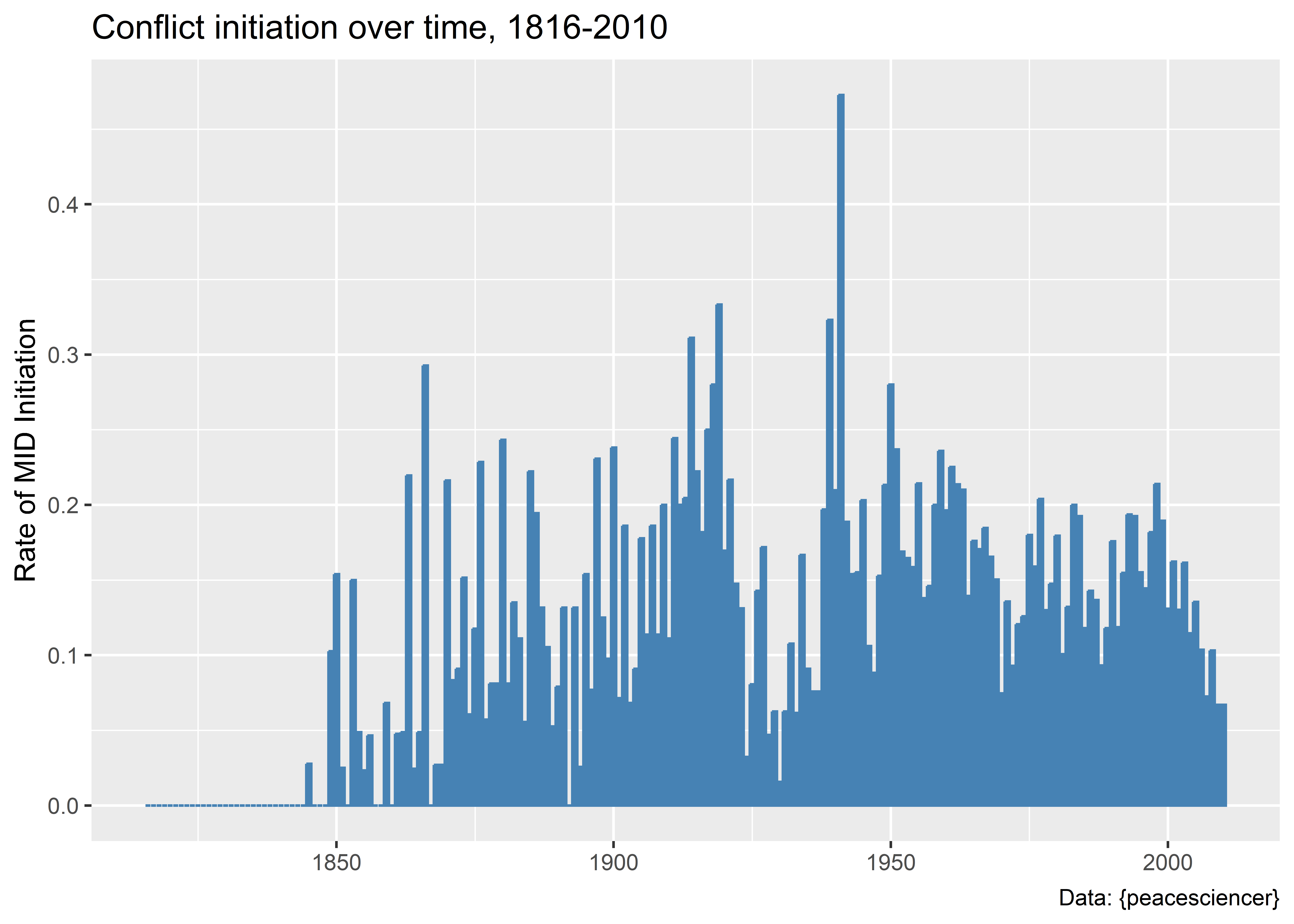
One of the advantages of using summarize() and group_by() in combination is that it makes plotting different summaries of your data so much easier. In a previous chapter we talked about how certain geom_*() functions with ggplot() will count and summarize things for you under the hood. This is fine in some cases, but sometimes the syntax necessary to make this happen isn’t terribly intuitive. Sometimes it will make more sense to do a combination of summarize() and group_by() with your data before using ggplot() to plot relationships. The below code shows an example of what this can look like. Notice that you can go from your full data, make a summary, and then give it the ggplot all within a series of pipes:
Data |>
  group_by(year) |>
  summarize(
    mean_mid_init = mean(gmlmidonset_init)
  ) |>
  ggplot() +
  aes(x = year, y = mean_mid_init) +
  geom_col(
    fill = "steelblue",
    color = "steelblue"
  ) +
  labs(
    x = NULL,
    y = "Rate of MID Initiation",
    title = "Conflict initiation over time, 1816-2010",
    caption = "Data: {peacesciencer}"
  )
7.6 Pivoting data with {tidyr}
There are some instances where we may want to pivot our data to make it longer or wider prior to plotting as well. This is useful, for example, if we want to conveniently show a trend in more than one variable over time in the same visualization. Say we wanted to compare what the frequency of conflict onset looks like over time compared to the rate. The frequency is just the raw count of new conflicts initiated, while the rate is the frequency divided by the total number of countries in the international system. One is an absolute measure that captures the overall level of conflict in the world, while the other is a measure of relative conflict risk.
We’ll start by creating a summary data object called mid_ts which shows, by year, the frequency and rate of new conflict initiation:
mid_ts <- Data |>
  group_by(year) |>
  summarize(
    total_mid_init = sum(gmlmidonset_init),
    mean_mid_init = mean(gmlmidonset_init)
  )
If we look at the data we can see that it gives us a data object with three columns:
mid_ts# A tibble: 195 × 3
year total_mid_init mean_mid_init
<dbl> <dbl> <dbl>
1 1816 0 0
2 1817 0 0
3 1818 0 0
4 1819 0 0
5 1820 0 0
6 1821 0 0
7 1822 0 0
8 1823 0 0
9 1824 0 0
10 1825 0 0
# ℹ 185 more rowsNow, without performing any other transformations do the data, we can give it directly to ggplot() for plotting. Since we want to see conflict frequency and rate side-by-side, we can just add a unique geom_line() layer for each:
ggplot(mid_ts) +
  aes(x = year) +
  geom_line(
    aes(y = total_mid_init),
    color = "navy"
  ) +
  geom_line(
    aes(y = mean_mid_init),
    color = "gray"
) 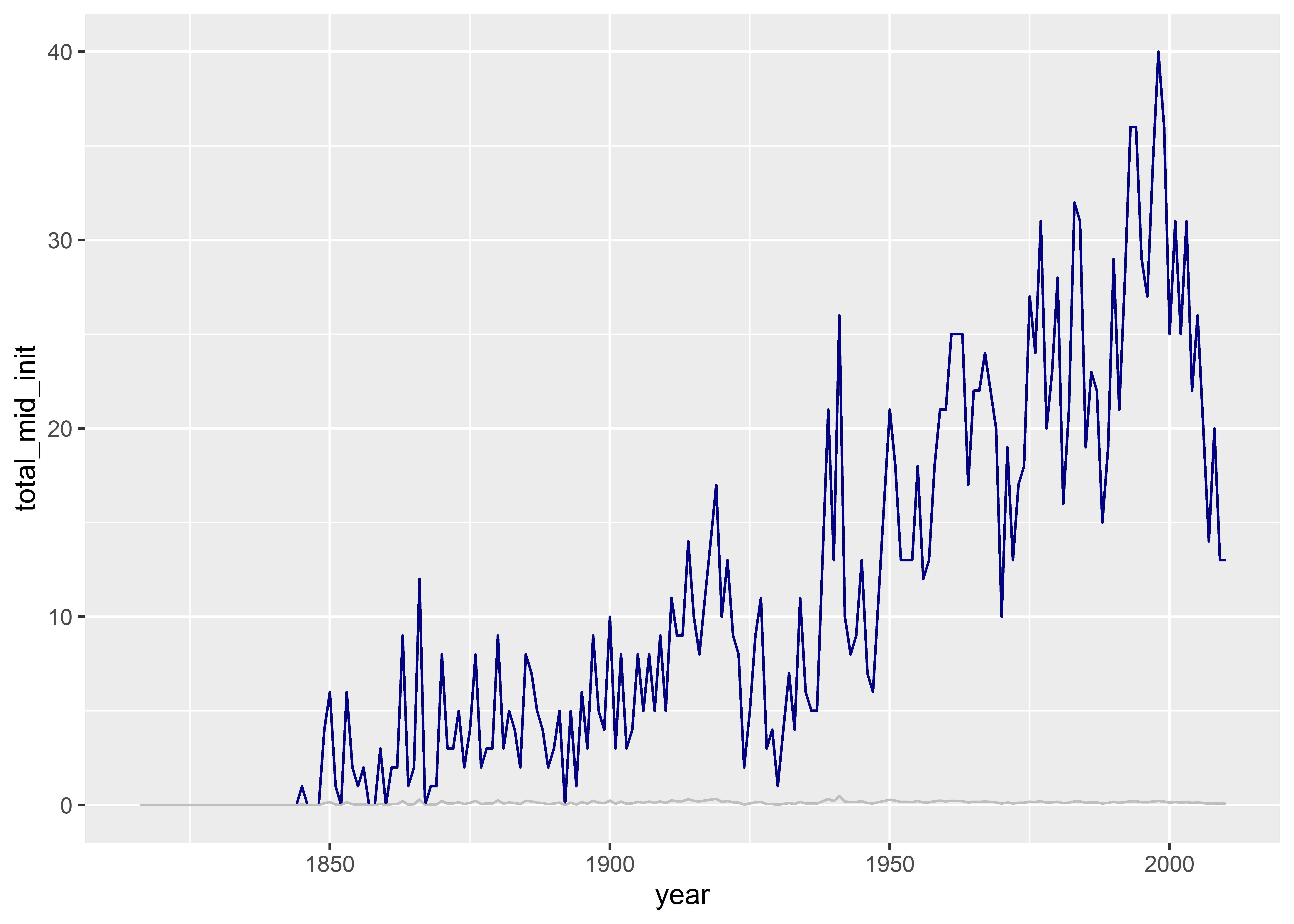
That’s was pretty simple, but the figure looks bad. It’s impossible to compare the frequency and the rate because they’re on different scales. We also don’t have a legend to indicate which line corresponds to which conflict measure. We can do this using a few hacks, but as a rule I like to avoid relying on too many of these. An alternative solution is to reshape our data and, then, to find a way to have a unique y-axis scale for each variable.
Enter the pivot functions. These live in the {tidyr} package, which, like {dplyr}, is part of the {tidyverse} and is opened automatically when you run library(tidyverse).
To help with plotting conflict trends using each of the measures we have in our dataset, the function we need to use is pivot_longer(). Here’s what it does to the data if we pivot longer on the conflict measures:
mid_ts |>
  pivot_longer(
    cols = total_mid_init:mean_mid_init
  )
# A tibble: 390 × 3
year name value
<dbl> <chr> <dbl>
1 1816 total_mid_init 0
2 1816 mean_mid_init 0
3 1817 total_mid_init 0
4 1817 mean_mid_init 0
5 1818 total_mid_init 0
6 1818 mean_mid_init 0
7 1819 total_mid_init 0
8 1819 mean_mid_init 0
9 1820 total_mid_init 0
10 1820 mean_mid_init 0
# ℹ 380 more rowsAs you can see above, I used pivot_longer() to reshape the dataset. In the process of doing this, I made it untidy. As a general rule of thumb, we like tidy data, which, if you remember, has three characteristics:
- Each row is an observation.
- Each column is a variable.
- Each cell has a single entry.
By pivoting the data, it no longer has characteristics 1 and 2. Though this is normally bad, it is actually ideal for plotting our data side-by-side with ggplot. This is because, with the data pivoted, we can do this:
mid_ts |>
  pivot_longer(
    total_mid_init:mean_mid_init
  ) |>
  ggplot() +
  aes(
    x = year,
    y = value
  ) +
  geom_line() +
  facet_wrap(~ name, scales = "free_y")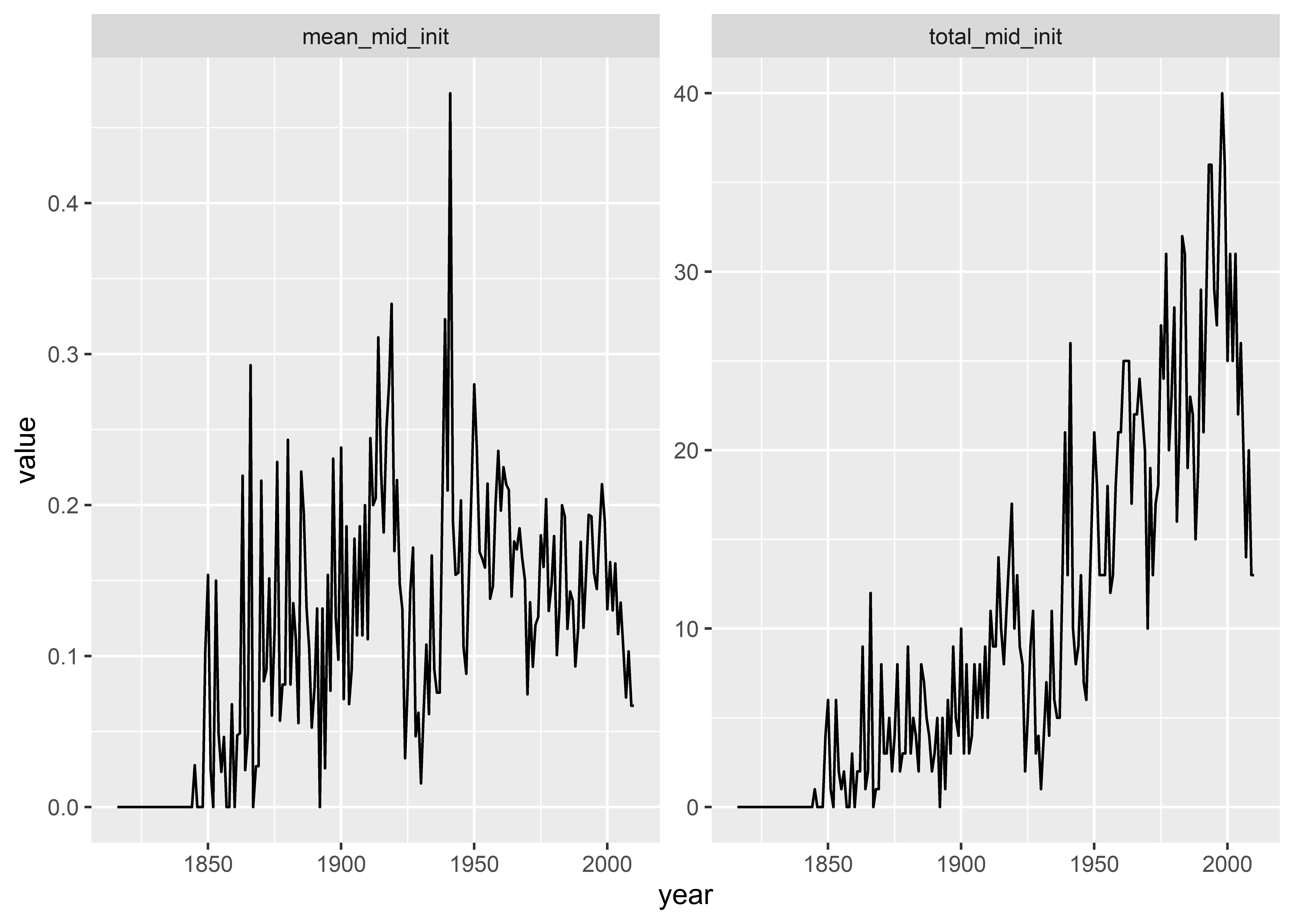
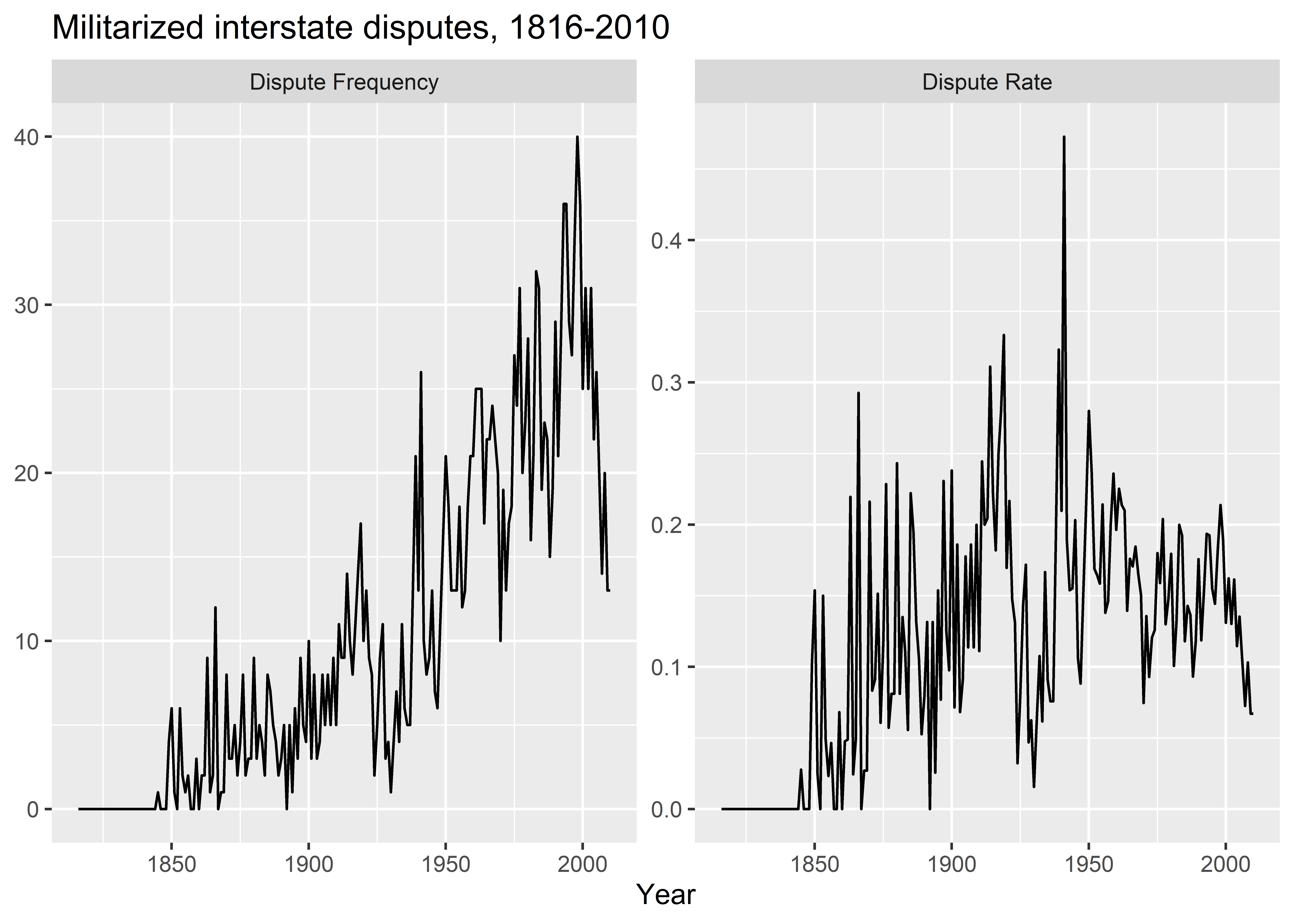
By pivoting the data, we produced our plot using much less code and we were able to make the plot a small multiple so that we can show the conflict rate and frequency by year on their own unique scales. We can do even more, though. The raw variable names don’t make great titles for the small multiples. We can fix this my using mutate() after pivoting the data. Check out the following code where I use a function called ifelse() to change the values in the name column. I also include an informative title and update the x- and y-axis titles.
mid_ts |>
  pivot_longer(
    total_mid_init:mean_mid_init
  ) |>
  mutate(
    name = ifelse(
      name == "total_mid_init",
      "Dispute Frequency",
      "Dispute Rate"
    )
  ) |>
  ggplot() +
  aes(
    x = year,
    y = value
  ) +
  geom_line() +
  facet_wrap(~ name, scales = "free_y") +
  labs(
    x = "Year",
    y = NULL,
    title = "Militarized interstate disputes, 1816-2010"
  )
7.7 Conclusion
Knowing how to properly use the data wrangling verbs discussed in this chapter will take time and plenty of practice. Don’t be discouraged if you struggle at first. If you can focus on just remembering what these verbs are and their purpose, you can work out the details of your code later. Sometimes just knowing the name of the function you want to use is 95% of the battle in programming.
Another tip that I think will be helpful is to remember to save the changes you make to your data. Say you use mutate() to make a new column in your data. If you run something like the following, the original data will be printed out with the new column sdppc, but it won’t be saved.
Data |>
  mutate(
    sdppc = exp(sdpest) / exp(wbpopest)
  )
If you want to ensure that your change to your data is saved you need to make sure you assign the output back to the name of your original data object:
Data |>
  mutate(
    sdppc = exp(sdpest) / exp(wbpopest)
  ) -> Data ## now it's saved in the data!
Something similar is true for other verbs that you apply to the data, but for certain changes you make be careful with how you save those changes. Sometimes it makes sense to assign the changes using the same object name that you started with. Other times, say if you filter the data, select only certain columns, or collapse it in some way you may want to save the changed data as a new object with a different name. Otherwise, your original dataset will be lost.
The big picture takeaway is (1) work on remembering what these different verbs are and what they do and (2) save changes to your data in a sensible way. If you can do these two things, you’ll go a long way in your ability to successfully wrangle all kinds of data.