## read in data from _data folder
library(tidyverse)
read_csv(
  here::here(
    "_data",
    "dataset.csv"
  )
) -> some_data3 Accessing Data and Making Your First Plot
3.1 Goals
Learning objectives:
- Get data into R
- Making a data visualization
- Cover some helpful resources if you want to go deeper into the details of using R
In this chapter, we’ll talk about a really important prerequisite for making data visualizations: accessing data! This may come as a surprise to you, but our software is not equipped to automatically produce plots with any dataset you wish to use. You have to make the data you intend to use known to R. We call this process reading in data, and there are many ways to read data into our environment (more than I can possibly cover in this chapter). Below, I walk through just a few of the most typical approaches that you’re likely to run into.
After we have some data to work with, we’ll then make our first data visualization. It won’t be anything fancy, but fanciness isn’t the goal. Rather, the goal is to briefly introduce the idea that reading in data and looking at said data go together.
Alright, let’s get to it…
3.2 Reading data into R
Data analysis is impossible without data (duh!), and the only way we can use data is to read it into R.
There are two main ways that I will have you access data in this class. The first is via spreadsheets (.csv or Google Sheets files) that are stored in some location—either in your files in the “_data” folder, on my GitHub, or in Google Drive. The second is via R packages that, once installed and opened, automatically populate your environment with one or several different datasets or specialized functions for querying and reading in datasets.
Let’s go over these different approaches.
3.2.1 Way 1: Reading in Files Stored in a Particular Location
The workhorse function we’ll use to read in files stored in some known location is read_csv() from the {readr} package, which is one of the many packages under the {tidyverse} umbrella.
When a file is local to your R project you can write some code like the following. Notice a few things about what I’ve written. First, I’m using read_csv(), and inside I’m using the here() function from the {here} package to help me navigate my R project files. Inside here() I first specify that I want R to go to my folder called “_data” and then to find a .csv file called “dataset.csv.” After making sure I’ve closed all parentheses () I then use reverse assignment and tell R to save the dataset I want to read in as an object called some_data (a really clever name). For any of the datasets stored in the “_data” folder, you can just update the below code with the appropriate file name and also change the name of the object you want the data to be saved as.
Sometimes, when people are nice, they make datasets publicly available at an online repository such as GitHub. I’ve done this for a bunch of different datasets that I’ve used over the years. To read in this data, you can use read_csv() as with the above code, but with one key difference. Rather than give read_csv() the location of a file in your R project, you’ll give it a url. Here’s what your code might look like in this scenario. In the below, I’ve created an object called the_url to which I’ve assigned the link to a raw .csv file on my GitHub in quotation marks (""). I’ve then given this object to read_csv() and saved the output as an object that, again, I’ve generically called some_data. I could have just given the url in quotation marks directly to read_csv(), but I prefer to separate it out like this.
the_url <-
  "https://raw.githubusercontent.com/milesdwilliams15/dpr-101-project-files/main/_data/election.csv"
read_csv(
  the_url
) -> some_data
Some datasets for this class will come from Google Drive. Here’s some example code for this scenario. Like the above example, I’m going to provide a link to the location of the data, but the difference now is that the dataset isn’t stored as a .csv file; it’s a .gsheet or Google Sheets file. read_csv() doesn’t know how to handle this kind of format, but there’s an R package called {googlesheets4} that has a function we can use instead. In the code below, I first save the url as an object. Then I open the {googlesheets4} library. Next, I use a function called gs4_deauth() which I run without giving it any input. When I run this function, it tells R that when I read in the data from Google Drive, it doesn’t need to get authentication using your gmail account and password. With that run, I then use a function called range_speedread() to read in the data from the Google spreadsheet and save it as an object called, yet again, some_data.
url <- "https://docs.google.com/spreadsheets/d/19RaIaVoJMChVsNGO45OrqZcSE3to-EwQ-vywngHLbks/edit#gid=817523709"
library(googlesheets4)
gs4_deauth()
range_speedread(
  url
) -> some_data
3.2.2 Way 2: R Packages
You’ll need to use one of the procedures above to read in many of the datasets you’ll use. However, some datasets come pre-installed in R, and some are accessible with different R packages. For example, the mtcars data frame is automatically accessible in R.
With other datasets you’ll need to use certain R packages that have been created to make it possible to access, query, and attach different datasets. Some example packages include {DemocracyData}, {peacesciencer}, and {socviz}. Say, for example, we wanted to access a dataset called election from the {socviz} package. All we would need to do is run the following code (and nothing more). Once you open the package, you’ll see a number of different data objects are now available in your environment, including election.
## open {socviz}
library(socviz)
3.3 From Reading in Data to Looking at Data
One of the first steps in data analysis (once our data is cleaned up of course) is data visualization. Looking at data can tell us a lot even before we do more formal analyses.
As an example, let’s use the election dataset from the {socviz} package:
library(socviz)We now have an object called county_data in our environment. This dataset contains information about county-level vote totals and shares for the 2012 and 2016 US Presidential elections, along with some other variables. Below, I’m using the sample_n() function to look at 10 random rows from the data (notice the use of the pipe operator |>):
county_data |>
  sample_n(10)
id name state census_region pop_dens pop_dens4
1 13023 Bleckley County GA South [ 50, 100) [ 45, 118)
2 55001 Adams County WI Midwest [ 10, 50) [ 17, 45)
3 18147 Spencer County IN Midwest [ 50, 100) [ 45, 118)
4 26013 Baraga County MI Midwest [ 0, 10) [ 0, 17)
5 37073 Gates County NC South [ 10, 50) [ 17, 45)
6 40113 Osage County OK South [ 10, 50) [ 17, 45)
7 51085 Hanover County VA South [ 100, 500) [118,71672]
8 21039 Carlisle County KY South [ 10, 50) [ 17, 45)
9 37041 Chowan County NC South [ 50, 100) [ 45, 118)
10 21011 Bath County KY South [ 10, 50) [ 17, 45)
pop_dens6 pct_black pop female white black travel_time land_area
1 [ 45, 82) [25.0,50.0) 12795 52.3 71.1 26.8 26.3 215.87
2 [ 25, 45) [ 2.0, 5.0) 20215 46.4 94.0 3.2 28.0 645.65
3 [ 45, 82) [ 0.0, 2.0) 20801 49.5 97.7 0.8 26.8 396.74
4 [ 9, 25) [ 5.0,10.0) 8654 45.2 74.1 7.5 16.3 898.26
5 [ 25, 45) [25.0,50.0) 11567 51.1 63.9 33.1 36.6 340.45
6 [ 9, 25) [10.0,15.0) 47981 49.7 66.3 11.5 24.0 2246.36
7 [215,71672] [ 5.0,10.0) 101918 51.0 86.9 9.6 25.3 468.54
8 [ 25, 45) [ 0.0, 2.0) 4978 51.3 96.5 1.2 25.6 189.43
9 [ 82, 215) [25.0,50.0) 14572 52.3 63.2 34.4 26.6 172.47
10 [ 25, 45) [ 0.0, 2.0) 12206 50.8 96.9 1.4 25.7 278.79
hh_income su_gun4 su_gun6 fips votes_dem_2016 votes_gop_2016
1 36073 [11,54] [12,54] 13023 1094 3717
2 44897 [ 8,11) [10,12) 55001 3780 5983
3 52991 [ 5, 8) [ 7, 8) 18147 2861 6572
4 41189 [11,54] [10,12) 26013 1156 2158
5 46592 [ 5, 8) [ 4, 7) 37073 2371 2851
6 44195 [11,54] [10,12) 40113 5593 12559
7 75070 [ 8,11) [ 8,10) 51085 19360 39592
8 39049 [11,54] [12,54] 21039 432 2094
9 34420 [ 5, 8) [ 4, 7) 37041 2965 3983
10 30797 [11,54] [12,54] 21011 1361 3082
total_votes_2016 per_dem_2016 per_gop_2016 diff_2016 per_dem_2012
1 4934 0.2217268 0.7533441 2623 0.2582093
2 10107 0.3739982 0.5919660 2203 0.5395109
3 9959 0.2872778 0.6599056 3711 0.4139846
4 3486 0.3316122 0.6190476 1002 0.4510029
5 5328 0.4450075 0.5350976 480 0.5169492
6 18942 0.2952698 0.6630240 6966 0.3737509
7 62313 0.3106896 0.6353730 20232 0.3102179
8 2599 0.1662178 0.8056945 1662 0.2863688
9 7108 0.4171356 0.5603545 1018 0.4723869
10 4577 0.2973563 0.6733668 1721 0.4294032
per_gop_2012 diff_2012 winner partywinner16 winner12 partywinner12 flipped
1 0.7313889 2320 Trump Republican Romney Republican No
2 0.4524018 894 Trump Republican Obama Democrat Yes
3 0.5670951 1489 Trump Republican Romney Republican No
4 0.5346705 292 Trump Republican Romney Republican No
5 0.4768362 213 Trump Republican Obama Democrat Yes
6 0.6262491 4523 Trump Republican Romney Republican No
7 0.6773449 21637 Trump Republican Romney Republican No
8 0.7006491 1085 Trump Republican Romney Republican No
9 0.5215517 365 Trump Republican Romney Republican No
10 0.5519165 505 Trump Republican Romney Republican NoUsing this data, we can make a simple scatter plot showing how the popular vote shares for the Republican Party are correlated with median house-hold income. We’ll do this using ggplot() from the {ggplot2} package, which is part of the {tidyverse}.
ggplot(county_data) +
  aes(x = hh_income, y = per_gop_2016) +
  geom_point()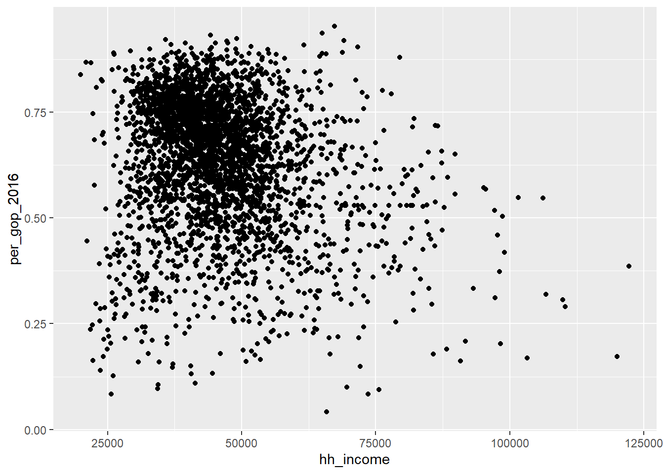
You should notice a few things about ggplot from the code used to produce the above figure. First, ggplot works by building figures in steps. We call these layers. Second, we add layers (literally) by using the + operator. While normally we use this for addition (i.e., 2 + 2) when we use ggplot the + acts a lot like a pipe operator (%>% or for later versions of R |>). Basically, the + in ggplot just tells R that we want to add a new set of commands or instructions for creating a plot.
More formally, the ggplot workflow looks like this:
- Feed ggplot data.
- Map aesthetics (tell ggplot what relationships to show).
- Draw geometry (tell ggplot how to show these relationships).
- Customize.
Back to the figure we made, as a first pass this is a bit spartan. We could obviously add a few more flourishes to make our data viz publication ready, but this is enough to get a sense for the data. Take a look at the figure. What does it tell us about house-hold income and support for Trump in 2016?
Another thing to note about making figures with ggplot() is that we can save them as objects in R. Check it out:
p <- ggplot(county_data) +
  aes(x = hh_income, y = per_gop_2016) +
  geom_point()
The object p is our ggplot data viz. Now, every time we write p, it tells R to produce the figure:
p
This feature of working with ggplot is great. The biggest benefit is that it lets us build up a solid foundation for a data viz and then add new details later.
For example, say we want to compare the above figure to a version where the scale for household income is different (say using the log-10 scale). All we need to do is add a new layer to p like so:
p + scale_x_log10()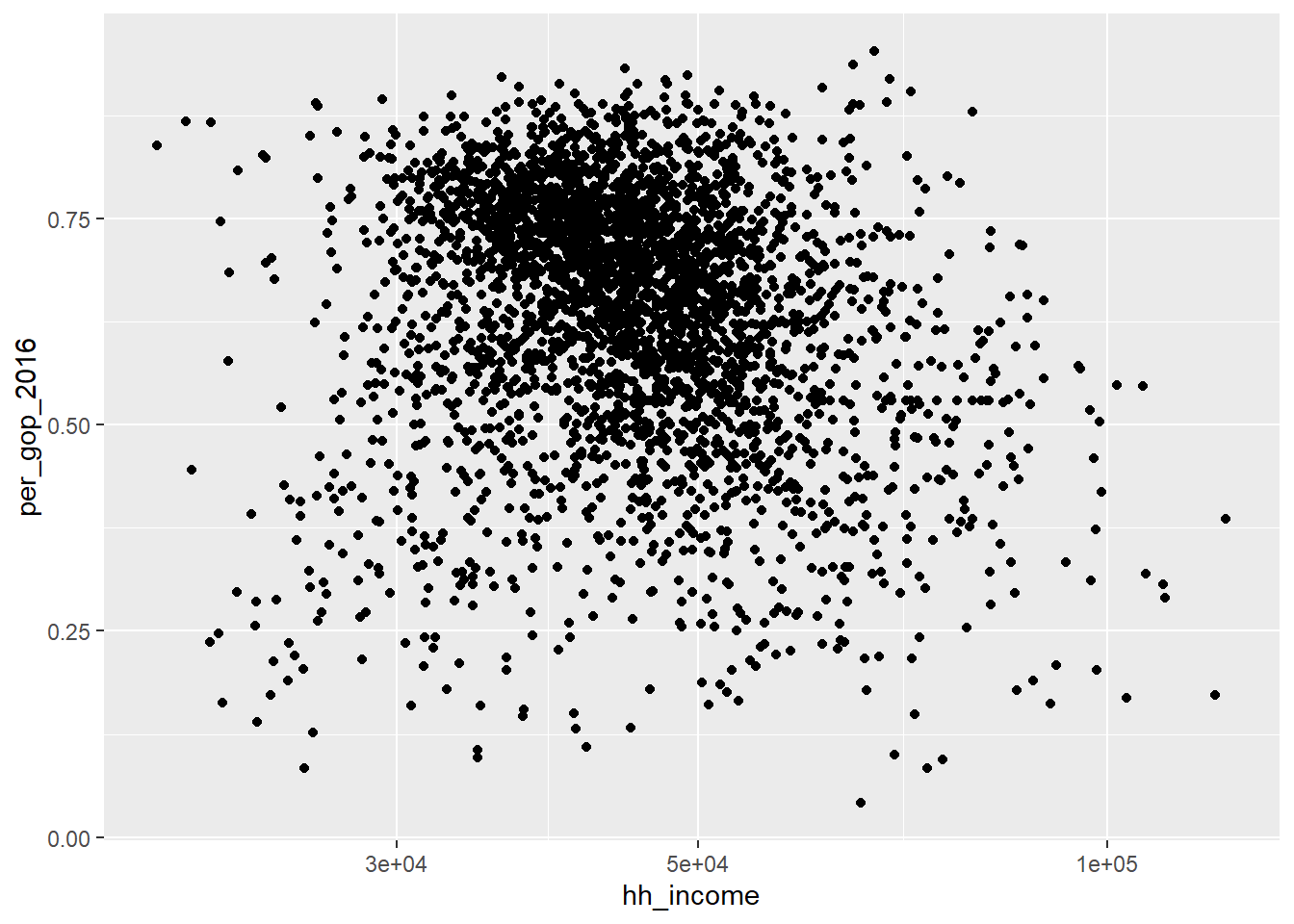
Because I saved the first plot as the object p, I didn’t have to re-write the code to produce the old plot before adding a new layer.
Speaking of this new layer, does the log-10 scale change any conclusions you previously drew about the data?
3.4 Helpful Resources for Learning More
This class is not about how to use R in its entirety, but you may find it helpful to get more familiar with it. Here are some resources for you to check out on your own time:
My personal favorite is swirlstats.com, because it lets you work at your own pace directly in R, and for free.
3.5 Wrapping up
Working with code is hard, and I promise you that you will run into problems. When you do, just remember that everyone has problems with their code—it’s normal, and it would be weird if you didn’t have any issues.
We’ll get more into the details of working with ggplot in the coming weeks. But for now, you should have at minimum some helpful examples for how to:
- Read data into R
- Make a basic plot using ggplot
- Access other resources for working in R