15  Dealing with Multiple Choice Survey Responses

What should you do when you have a survey question that lets people enter multiple choices? When this happens, you may see in the survey data the question number associated with this (something like q14) followed by an underscore and a series of additional numbers (like q14_1, q14_2, etc.).

Your first instinct when dealing with these questions is probably to turn each of the columns into a single factor that indicates how people responded to each unique option in this multiple response question. The problem with this approach is that there are many possible combinations of responses individuals could have given. A better approach is to keep these responses as separate columns. It’s actually better to treat them like unique questions that just happen to be related.

Now, keeping these questions separate doesn’t mean you have to analyze them individual as well when you get to your data visualization. Actually, it’s a good idea to look at them together. But since these are separate responses, you’ll need to use some of the tools we talked about with “data wrangling.” Specifically, pivot_longer().

Let’s get to it.

15.1 Cleaning multiple response questions

Every semester, Data for Political Research at Denison University surveys the student body, asking them questions about a bunch of things, including their major area of study, study habits, and politics. Some questions are straightforward, like which political party do you identify with. These questions only let students pick one option in their response. Other questions, however, let students select many different options.

A good example of this is question 23 in the March 2024 wave of the DU student survey. It asks students what division their major is in. There are five academic divisions they can chose from, plus a sixth “undecided” option.

While students who took the survey were presented with this question as though it were a single question, in the survey data responses are broken up into six columns where 1 means a student selected that division and NA means they did not. The below code reads in the data, which is saved as a Google sheet on Google Drive. It then selects the question 23 columns and shows the first six rows of the data to show what they look like. All we have are a bunch of 1s and NAs.

## open packages
library(tidyverse)
library(socsci)
library(googlesheets4)

## read in the data (March 2024 DU survey)
gs4_deauth()
range_speedread(
  "https://docs.google.com/spreadsheets/d/1qq5VkNDzFonfEiRxf03NHvktzMsQNOWCzkXdkvkw9E8/edit"
) -> Data

## show Q23 responses
Data |>
  select(
    starts_with("Q23_")
  ) |>
  slice_head(n = 6)

# A tibble: 6 × 6
  Q23_1 Q23_2 Q23_3 Q23_4 Q23_5 Q23_6
  <dbl> <dbl> <dbl> <dbl> <dbl> <dbl>
1    NA     1    NA    NA    NA    NA
2    NA     1     1    NA    NA    NA
3    NA    NA    NA    NA     1    NA
4    NA     1    NA    NA    NA    NA
5    NA    NA     1    NA     1    NA
6    NA     1    NA    NA    NA    NA

There’s a really simple solution to this problem. As noted at the outset, even though Q23 is presented to students as a single question, for the purposes of analysis it makes good sense to treat these responses as six separate variables. That means all we need to do to prep the data is turn all the NAs into 0s. By doing this, we are turning these Q23 responses into a set of academic division “dummy variables.” The below code uses a combination of mutate() and across() to apply the necessary transformation across all six of these columns.

## update Q23 responses so that NAs == 0
Data |>
  mutate(
    across(
      starts_with("Q23_"),
      ~ replace_na(.x, 0)
    )
  ) -> Data

Just to check that the code worked, we can take a look at the data again:

## show Q23 responses
Data |>
  select(
    starts_with("Q23_")
  ) |>
  slice_head(n = 6)

# A tibble: 6 × 6
  Q23_1 Q23_2 Q23_3 Q23_4 Q23_5 Q23_6
  <dbl> <dbl> <dbl> <dbl> <dbl> <dbl>
1     0     1     0     0     0     0
2     0     1     1     0     0     0
3     0     0     0     0     1     0
4     0     1     0     0     0     0
5     0     0     1     0     1     0
6     0     1     0     0     0     0

15.2 Visualizing multiple response questions

Even though we’ll treat these questions as separate variables, there’s no denying that they’re related. This means we should probably analyze them together. But what’s a convenient way to do this? Enter pivot_longer().

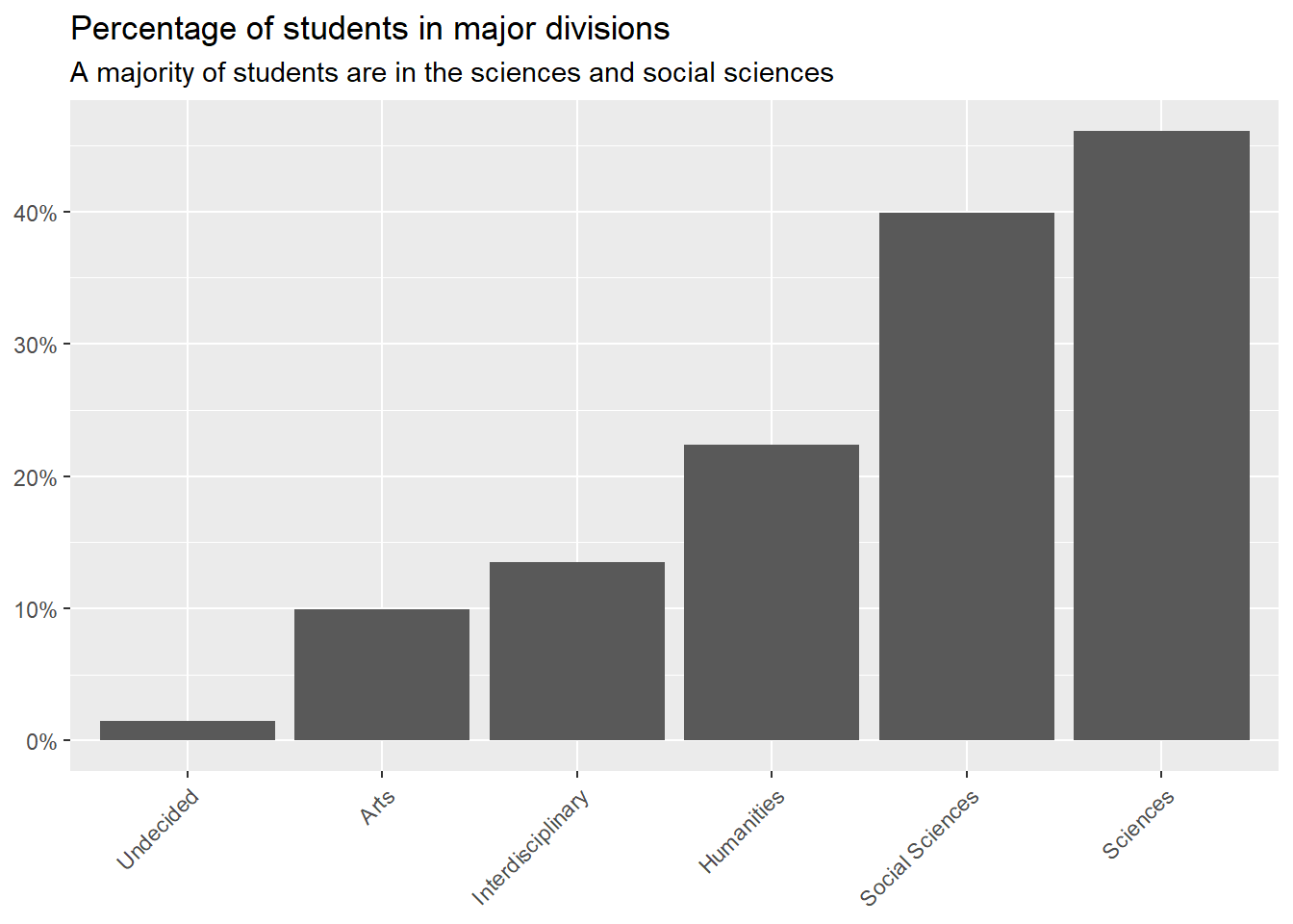
If you remember from our notes on data wrangling, pivot_longer() is a useful tool for taking a tidy dataset and making it untidy, but in a useful way for data visualization. Here’s some code that uses pivot_longer() with Q23 responses to help summarize the distribution of students who report having a major in one of the five different academic divisions at Denison or else are “undecided.” The figure produced includes an informative title and subtitle that tell us what the figure is showing us. In particular, it’s telling us that a majority of students are in the sciences and social sciences.

## summarize the responses to these questions
Data |>
  pivot_longer(
    starts_with("Q23_")
  ) |>
  mutate(
    name = rep(
      c("Social Sciences",
        "Sciences",
        "Humanities",
        "Arts",
        "Interdisciplinary",
        "Undecided"),
      len = n()
    )
  ) |>
  group_by(name) |>
  ct(value) |>
  filter(value == 1) |>
  ggplot() +
  aes(
    x = reorder(name, pct),
    y = pct
  ) +
  geom_col() +
  labs(
    x = NULL,
    y = NULL,
    title = "Percentage of students in major divisions",
    subtitle = "A majority of students are in the sciences and social sciences"
  ) +
  scale_y_continuous(
    labels = scales::percent
  ) +
  theme(
    axis.text.x = element_text(
      angle = 45,
      hjust = 1
    )
  )

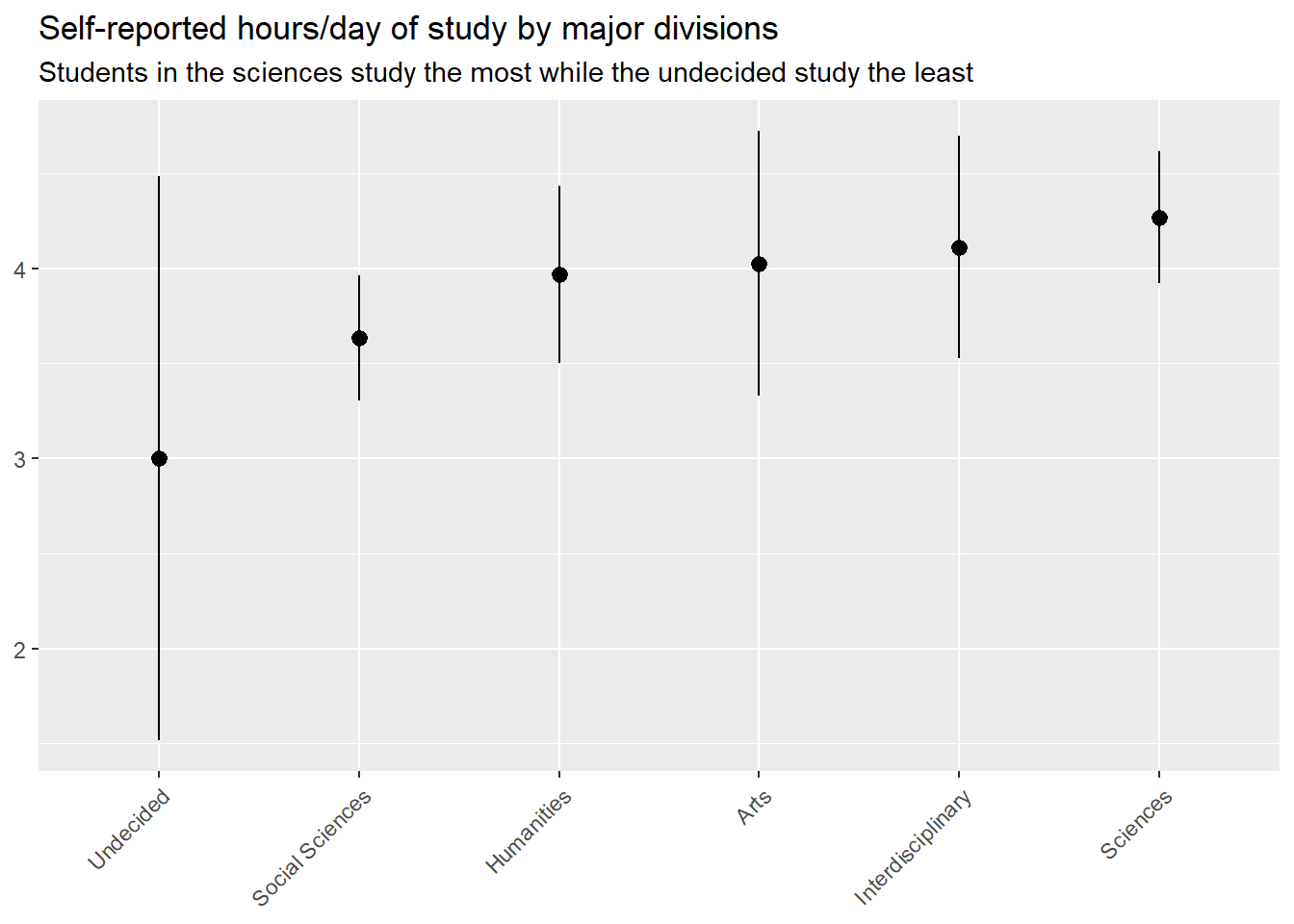
We can use pivot_longer() to help us show the distribution of other variables in the data by academic division as well. The below code does this with responses to Q24_2, which indicates students’ self-reported hours per day spent studying for their longest class day. Students in the sciences appear to study the most, while those still undecided are studying the least.

## use these responses to explain other variables
Data |>
  pivot_longer(
    starts_with("Q23_")
  ) |>
  mutate(
    name = rep(
      c("Social Sciences",
        "Sciences",
        "Humanities",
        "Arts",
        "Interdisciplinary",
        "Undecided"),
      len = n()
    )
  ) |>
  group_by(name, value) |>
  mean_ci(Q24_2) |>
  filter(value == 1) |>
  ggplot() +
  aes(
    x = reorder(name, mean),
    y = mean,
    ymin = lower,
    ymax = upper
  ) +
  geom_pointrange() +
  labs(
    x = NULL,
    y = NULL,
    title = "Self-reported hours/day of study by major divisions",
    subtitle = "Students in the sciences study the most while the undecided study the least"
  ) +
  theme(
    axis.text.x = element_text(
      angle = 45,
      hjust = 1
    )
  )

15.3 Conclusion

Multiple response questions are common in surveys, so knowing how to handle them is a necessary skill. Most of the time, the best approach is to treat all the unique responses to these questions as separate responses for the purposes of cleaning your data and then to analyze them together by pivoting your data to produce unique summaries for each response.

A little bonus with this approach is that you can also study how these responses are correlated as well. For example, you could look at how often students in the sciences also have a major in the arts.