# this is a comment that won't run any code
1 + 3 # this is some code that will run (but this comment won't)[1] 4# 1 + 3Learning objectives:
In this R Companion we’ll use R and Posit Workbench (formerly RStudio) for data analysis. Before we get started, it’s essential that you familiarize yourself with the Posit environment.
First, access the R server and log-in with your Denison credentials. If you’re off campus, you’ll need a VPN connection to access the server. You can read more about how to do that via one of the following links:
Once you access the server, you may already be in a project space. If not, you’ll need to start a new session.
In the Workbench environment you should see few different components, including:
At this point you should be able to tell that a lot is going on in the Workbench. You’re looking at what’s called an “integrated development environment” (IDE) that actually is a language-agnostic application separate from R itself. Within the workbench, you can use R, Python, or SQL, among other languages as well. R is pretty spartan all on its own, and it definitely falls short as far as user-friendly software goes. The workbench provides a better interface with R proper that lets you organize files, save your work in projects, and write reports within a single environment. And as you learn additional languages, like Python, you can keep using the workbench and (even better) Quarto files to save your work.
The best way to organize your work is to save it in projects. This way all of your data, code, and notes related to a single project can live in one place.
If you look at the upper right corner, you can see a cube with an “R” in it. If you select that you’ll see a drop-down menu. Select “New Project” > “New Directory” > “New Project” > enter a new directory name for your project > use “brows” to find a place in your files you’d like to save your work > then create. For this class, I recommend creating a project called “DPR 201” that way it’s obvious to your future self that this is where your work for this class is located.
After you create your project, create two new folders in your files. Call one “Data” and the other “Code.” One will be where you save different datasets you use in this class. The other will be where you save the Quarto files you use in this class for notes and course assignments.
Quarto documents are a great place to
You can also use these documents to write reports, but we’ll talk more about that later.
These features of working in Quarto are great for learning to code. You can make notes to yourself using a visual editor (similar to a word doc, but with some extra bells and whistles) about what data you’re working with and what your code is supposed to be doing.
There are lots of helpful resources out there for working with Quarto. I recommend starting with the main Quarto page.
When you work with Quarto, you can either work in the source version of the document, or the visual version. The latter is a visual editor of a Quarto document that makes it really easy and intuitive to create section headers, use different font faces, and drop in code chunks. I recommend using the visual editor.
To turn your document into a report, you can use the “Render” button at the top (the one that has the big blue arrow).
When you render something, you can update a few things about how it renders. For example, if you want to hide all of the code in your code chunks while only letting the output appear in your rendered document, you can write the following as your first code chunk in your document:
#| echo: false
knitr::opts_chunk$set(echo = FALSE)When you use Quarto, your notes/comments/writing in plain text will be interspersed with R code bocks.
An Rcode block is created using three backticks (“```”) followed by an “r” in brackets, and then it’s closed with three more backticks.
Think of each code block as a self-contained space for writing and running a specific bit of code. After you make a code block and write some code in it, you have a bunch of different options for running it.
In addition to making notes in plain text around your code chunks, you can make notes inside code chunks as well. Anything that follows a # in a bit of R code is “commented out.” That means R knows not to run anything that follows the hashtag in the code. For example:
# this is a comment that won't run any code
1 + 3 # this is some code that will run (but this comment won't)
[1] 4# 1 + 3You can use a hashtag-vertical line combo to give specific preferences for how a given code block runs.
Say you don’t want a particular code block to appear in a rendered document. You would write the following message indicating echo should be false followed by the code you want to run.
#| echo: false
2 + 2
You can also include a label if you’re producing a data visualization. Here’s a very simple example:
#| fig-cap: "An example figure with a label"
plot(mtcars$wt, mtcars$mpg)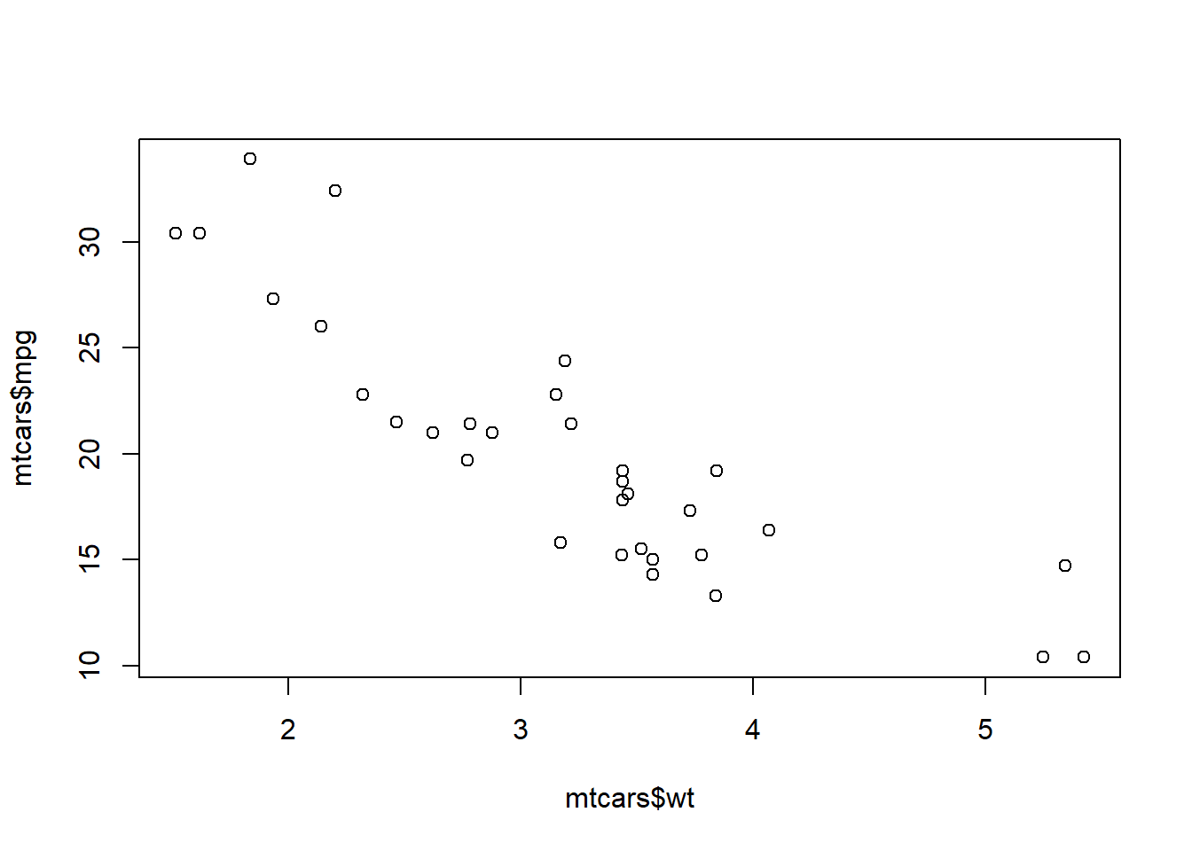
There are few things to know about R. First and foremost, R is a language. And just like any language, fluency in R takes time and a lot of practice.
R specifically is an “object oriented” and “functional” programming language. That means a few things.
First, everything in R has a name. You refer to the names of things to examine them or use them. These things can be variables or datasets that you manipulate, or functions that you use to perform operations.
Like any language, there are some grammatical rules in R that you should never break (and cannot break if you tried). For example, words like TRUE or FALSE, Inf or else, and several others have been reserved for core programming purposes and you couldn’t name something in R one of these things if you tried.
Other words or letters, like q, c, or mean can technically be used to refer to other things, but avoid doing so! These are the names of basic functions in R, and if you give other things in R the same names, R will get confused and angry with you.
R is also case sensitive. So if something is named This R won’t know what you’re talking about if you try to call This by instead writing this.
Second, everything in R is an object.
Say we use the command c(), which is a function that stands for “concatenate.” It takes a sequence of commands and returns a vector where each element is accessible:
c(1, 2, 4, 8, 16, 32)[1] 1 2 4 8 16 32The output from the above is just all the elements in the vector we created using c(). If we didn’t want this to just appear in the console but instead have it saved, we would need to assign the vector a name, which then saves it as an object:
my_numbers <- c(1, 2, 4, 16, 32)Now, every time we call the object my_numbers, the output will appear in the console (or as the output of a code block):
my_numbers[1] 1 2 4 16 32Each of the numbers in this vector can be accessed directly, too. This is done using square brackets [] after the name of the object:
my_numbers[3][1] 4The above prints the 3rd element in the vector called my_numbers.
We created my_numbers using an assignment operator <-. When you want to save something as an object, you need to use an assignment operator. A neat feature of R is that assignment can operate in two directions; not only from the right to the left (the usual way), but also from the left to the right. The latter is sometimes called “reverse assignment.” Here’s an example using both:
# normal assignment
x <- c(1, 2, 3)

# reverse assignment
c(4, 5, 6) -> y
You can technically use the = operator to assign things, too, but there are some things to note about this:
Generally, it’s considered bad grammar to use = for assignment. Instead, we use = inside of functions (coming up next) to set commands or feed objects to functions when we want to perform an operation.
Speaking of functions, just about everything you do in R with be with a function. A function is a special kind of object that performs actions for you. You feed it some kind of input (like an object) and it provides an output (which you can assign to a new object for later use).
For example, there’s a function called mean() which we can use on the object my_numbers:
mean(x = my_numbers)[1] 11Notice the use of x = my_numbers inside the ( ). Since mean() expects that the first input it receives is a set of values to calculate the mean of, you can also just write:
mean(my_numbers)[1] 11The function does exactly what its name suggests—it returns the mean or average of whatever numerical vector you feed it.
However, like all functions, mean() has some rules about what kinds of inputs it will accept.
If you feed it nothing, it’ll give you an error that says Error in mean.default() : argument "x" is missing, with no default
If you feed it non-numerical data, it’ll give you a warning and return NA:
my_words <- c("Hello", "World!")
mean(my_words)
Warning in mean.default(my_words): argument is not numeric or logical: returning
NA[1] NAWhat’s the average of “Hello” and “World!” I dunno, and neither does your computer.
If you ever want to learn more about a function, each function in R has a help file. All you need to do to access the help file for a particular function is write something like help(function_name) in the console. You could just write ?function_name in the console as well.
An important thing to note about functions is that they come in packages. Some functions, like mean(), are in the {baseR} package which is already open and ready to go the moment you open R. By the way, any time we refer to a package in R in plain text, we the convention is to include squiggly brackets around the package name—e.g., {packagename}.
While the {baseR} package is automatically opened once you start an R session, you’ll usually need to explicitly tell R you want to open other packages. You’ll do this with the library() function. In a code chunk, just write library(packagename) to open the package.
In this class, we’ll use the {tidyverse} of R packages. The tidyverse is actually a package of packages that have functions that are meant to be used together. Rather than attach each package in the tidyverse individually, if we write library(tidyverse) all these packages and the functions they contain are immediately accessible to us.
library(tidyverse)Some packages have already been pre-installed for you if you’re using the Denison server. If you aren’t, you’ll need to install these using the install.packages() function.
Also note that some packages have been produced by users and aren’t yet accessible from the “CRAN.” For these functions, you have to take some additional steps to install the package.
One in particular is the {coolorrr} package that I personally created to make working with color palettes in figures easier. To install it, you’ll need to run the following in your console:
devtools::install_github("milesdwilliams15/coolorrr")Notice in the above that I used double colons :: after devtools. If you ever only want to access a single function from a package ({devtools} is a package that helps with installing packages from sources like GitHub), but don’t want to attach the full package in R, you can write the package name followed by :: to call the function you want. The syntax will be something like packagename::functionname().
R is many things, including a glorified calculator. You can use a lot of different operations like * for multiplication, / for division, + for addition, and - for subtraction.
R also uses a number of logical operators like and &, or |, not !, equal to ==, greater than >, greater than or equal to >=, less than <, less than or equal to <=, not equal to !=, and in %in%.
Remember the x and y objects I created earlier? Let’s try out some of these operations on them and see what happens:
# Mathematical operations
x + y # addition
[1] 5 7 9x - y # subtraction[1] -3 -3 -3x * y # multiplication[1] 4 10 18x / y # division[1] 0.25 0.40 0.50# Logical operations
x == y # equivalence[1] FALSE FALSE FALSEx <= y # x less than or equal to y?[1] TRUE TRUE TRUEx %in% y # are x values in y?[1] FALSE FALSE FALSENotice that mathematical operators return numerical outputs, while logical operators return logical outputs (TRUE or FALSE).
Note that R treats logical values as 0-1 values. For example, you can take the mean of a vector of TRUE and FALSE values:
mean(c(0, 1))[1] 0.5mean(c(F, T)) # these are the same[1] 0.5You can also just write T for TRUE and F for false, as I did in the above block.
Another feature of R (at least for more recent versions) is a the base R “pipe” operator |>. This operator lets you tell R you want to give some object to a particular function, like so:
x |>
  mean()
[1] 2This might seem unnecessary, but this ability to pipe from one object to some function comes in handy when you want to perform many different sets of operations in succession.
Most of the work we do in this class will involve working with datasets. Think of these as tables that store data in a central location for ease of access and use.
mtcars is a dataset that already comes pre-installed in R. We can check out the first 10 rows of the data using the head() function:
head(mtcars, 10) mpg cyl disp hp drat wt qsec vs am gear carb
Mazda RX4 21.0 6 160.0 110 3.90 2.620 16.46 0 1 4 4
Mazda RX4 Wag 21.0 6 160.0 110 3.90 2.875 17.02 0 1 4 4
Datsun 710 22.8 4 108.0 93 3.85 2.320 18.61 1 1 4 1
Hornet 4 Drive 21.4 6 258.0 110 3.08 3.215 19.44 1 0 3 1
Hornet Sportabout 18.7 8 360.0 175 3.15 3.440 17.02 0 0 3 2
Valiant 18.1 6 225.0 105 2.76 3.460 20.22 1 0 3 1
Duster 360 14.3 8 360.0 245 3.21 3.570 15.84 0 0 3 4
Merc 240D 24.4 4 146.7 62 3.69 3.190 20.00 1 0 4 2
Merc 230 22.8 4 140.8 95 3.92 3.150 22.90 1 0 4 2
Merc 280 19.2 6 167.6 123 3.92 3.440 18.30 1 0 4 4This is a “dataframe,” or what we might also call a dataset.
To access a single column of a dataframe, just use the syntax dataset$variable:
mtcars$mpg [1] 21.0 21.0 22.8 21.4 18.7 18.1 14.3 24.4 22.8 19.2 17.8 16.4 17.3 15.2 10.4
[16] 10.4 14.7 32.4 30.4 33.9 21.5 15.5 15.2 13.3 19.2 27.3 26.0 30.4 15.8 19.7
[31] 15.0 21.4A particularly useful way to save a dataframe in R is as a tibble. To convert a dataframe to a tibble (which is a special kind of dataframe) just write:
mtcars_tb <- as_tibble(mtcars)
head(mtcars_tb, 10)
# A tibble: 10 × 11
mpg cyl disp hp drat wt qsec vs am gear carb
<dbl> <dbl> <dbl> <dbl> <dbl> <dbl> <dbl> <dbl> <dbl> <dbl> <dbl>
1 21 6 160 110 3.9 2.62 16.5 0 1 4 4
2 21 6 160 110 3.9 2.88 17.0 0 1 4 4
3 22.8 4 108 93 3.85 2.32 18.6 1 1 4 1
4 21.4 6 258 110 3.08 3.22 19.4 1 0 3 1
5 18.7 8 360 175 3.15 3.44 17.0 0 0 3 2
6 18.1 6 225 105 2.76 3.46 20.2 1 0 3 1
7 14.3 8 360 245 3.21 3.57 15.8 0 0 3 4
8 24.4 4 147. 62 3.69 3.19 20 1 0 4 2
9 22.8 4 141. 95 3.92 3.15 22.9 1 0 4 2
10 19.2 6 168. 123 3.92 3.44 18.3 1 0 4 4There are lots of ways for peering into a dataset/dataframe to get a sense for its structure (what it contains, how big it is, etc.).
You can use summary() to get some quick summary statistics that tell you about the variables in a dataset:
summary(mtcars_tb) mpg cyl disp hp
Min. :10.40 Min. :4.000 Min. : 71.1 Min. : 52.0
1st Qu.:15.43 1st Qu.:4.000 1st Qu.:120.8 1st Qu.: 96.5
Median :19.20 Median :6.000 Median :196.3 Median :123.0
Mean :20.09 Mean :6.188 Mean :230.7 Mean :146.7
3rd Qu.:22.80 3rd Qu.:8.000 3rd Qu.:326.0 3rd Qu.:180.0
Max. :33.90 Max. :8.000 Max. :472.0 Max. :335.0
drat wt qsec vs
Min. :2.760 Min. :1.513 Min. :14.50 Min. :0.0000
1st Qu.:3.080 1st Qu.:2.581 1st Qu.:16.89 1st Qu.:0.0000
Median :3.695 Median :3.325 Median :17.71 Median :0.0000
Mean :3.597 Mean :3.217 Mean :17.85 Mean :0.4375
3rd Qu.:3.920 3rd Qu.:3.610 3rd Qu.:18.90 3rd Qu.:1.0000
Max. :4.930 Max. :5.424 Max. :22.90 Max. :1.0000
am gear carb
Min. :0.0000 Min. :3.000 Min. :1.000
1st Qu.:0.0000 1st Qu.:3.000 1st Qu.:2.000
Median :0.0000 Median :4.000 Median :2.000
Mean :0.4062 Mean :3.688 Mean :2.812
3rd Qu.:1.0000 3rd Qu.:4.000 3rd Qu.:4.000
Max. :1.0000 Max. :5.000 Max. :8.000 You can use the glimpse() function to check the data’s structure:
glimpse(mtcars_tb)Rows: 32
Columns: 11
$ mpg <dbl> 21.0, 21.0, 22.8, 21.4, 18.7, 18.1, 14.3, 24.4, 22.8, 19.2, 17.8,…
$ cyl <dbl> 6, 6, 4, 6, 8, 6, 8, 4, 4, 6, 6, 8, 8, 8, 8, 8, 8, 4, 4, 4, 4, 8,…
$ disp <dbl> 160.0, 160.0, 108.0, 258.0, 360.0, 225.0, 360.0, 146.7, 140.8, 16…
$ hp <dbl> 110, 110, 93, 110, 175, 105, 245, 62, 95, 123, 123, 180, 180, 180…
$ drat <dbl> 3.90, 3.90, 3.85, 3.08, 3.15, 2.76, 3.21, 3.69, 3.92, 3.92, 3.92,…
$ wt <dbl> 2.620, 2.875, 2.320, 3.215, 3.440, 3.460, 3.570, 3.190, 3.150, 3.…
$ qsec <dbl> 16.46, 17.02, 18.61, 19.44, 17.02, 20.22, 15.84, 20.00, 22.90, 18…
$ vs <dbl> 0, 0, 1, 1, 0, 1, 0, 1, 1, 1, 1, 0, 0, 0, 0, 0, 0, 1, 1, 1, 1, 0,…
$ am <dbl> 1, 1, 1, 0, 0, 0, 0, 0, 0, 0, 0, 0, 0, 0, 0, 0, 0, 1, 1, 1, 0, 0,…
$ gear <dbl> 4, 4, 4, 3, 3, 3, 3, 4, 4, 4, 4, 3, 3, 3, 3, 3, 3, 4, 4, 4, 3, 3,…
$ carb <dbl> 4, 4, 1, 1, 2, 1, 4, 2, 2, 4, 4, 3, 3, 3, 4, 4, 4, 1, 2, 1, 1, 2,…Every time you’re done working, make sure you do a few things:
You should always perform the above three steps when you close out (with special emphasis placed on step 2). This ensures R is always running smoothly and efficiently.
Be patient with yourself as you start working in R and the Posit Workbench/RStudio IDE. At the same time that you are familiarizing yourself with new software, you also are learning to speak a new language. If things don’t make sense at first, that’s okay. That’s normal.
I can’t possibly anticipate every possible issue you may run into as you use R, but I can give you a heads up about some common mistakes people make:
> at the bottom of the console, all is good. If you see a + then something only partially ran.x, then ran a function on it and saved the output as x, then tried to go back and run an old chunk on x only to find that it spits out an error. The old x that used to work with a function now no longer does because the new x isn’t the same thing!