3Prerequisites II: Accessing Data and Making Plots
3.1 Goals
Get data into R
Making a data visualization
Cover some helpful resources if you want to go deeper into the details of using R
3.2 Reading data into R
Data analysis is impossible without data. The only way we can use data is to get it into R.
A lot of packages (including base R) provide tools for reading data into R. In this class, we’ll primarily use the read_csv() function from the {readr} package. This is one of the many packages in the {tidyverse} ecosystem of packages.
There are three main ways that I will have you access data in this class. The first is via .csv files I have stored on my GitHub. The second is on Google Drive. The third is using R packages that have been developed to specifically pull data from different online databases.
To read the data into R, we can use the read_csv() function like so:
library(tidyverse)
Warning: package 'tidyverse' was built under R version 4.2.3
Warning: package 'ggplot2' was built under R version 4.2.3
Warning: package 'tibble' was built under R version 4.2.3
Warning: package 'tidyr' was built under R version 4.2.3
Warning: package 'readr' was built under R version 4.2.3
Warning: package 'purrr' was built under R version 4.2.3
Warning: package 'dplyr' was built under R version 4.2.3
Warning: package 'stringr' was built under R version 4.2.3
Warning: package 'forcats' was built under R version 4.2.3
Warning: package 'lubridate' was built under R version 4.2.3
── Attaching core tidyverse packages ──────────────────────── tidyverse 2.0.0 ──
✔ dplyr     1.1.2     ✔ readr     2.1.4
✔ forcats   1.0.0     ✔ stringr   1.5.0
✔ ggplot2   3.5.0     ✔ tibble    3.2.1
✔ lubridate 1.9.3     ✔ tidyr     1.3.0
✔ purrr     1.0.2
── Conflicts ────────────────────────────────────────── tidyverse_conflicts() ──
✖ dplyr::filter() masks stats::filter()
✖ dplyr::lag()    masks stats::lag()
ℹ Use the conflicted package (<http://conflicted.r-lib.org/>) to force all conflicts to become errors
Data <-read_csv("https://raw.githubusercontent.com/milesdwilliams15/Teaching/main/DPR%20101/Data/onset_and_wgi.csv")
Rows: 3047 Columns: 4
── Column specification ────────────────────────────────────────────────────────
Delimiter: ","
chr (1): country
dbl (3): year, sumonset1, wgi

ℹ Use `spec()` to retrieve the full column specification for this data.
ℹ Specify the column types or set `show_col_types = FALSE` to quiet this message.
Notice that I used quotation marks ("") around the url. Some things in R require the use of quotation marks (like data files or character strings) and other things don’t (like the names of objects or functions).
Importantly, when read_csv() reads the data into R, it will spit out a few messages when it’s done. These provide details about how read_csv() assigned variable classes to each of the columns in the data. In this case, it tells us that it assigned country to the character class (that means it’s a non-ordered category) and it assigned year, sumonset1, and wgi the class double, which is R’s way of saying real numbers.
3.2.2 Way 2: Local Files in Your Project “Data” Folder
You can give read_csv() a url like I did above, or the location of a file stored elsewhere. For example, I’m writing this note on my laptop, and the same dataset I have on my GitHub also lives in my files on my computer. To access it locally, I could use the here() function from the {here} package to tell R where to pull the data from:
You don’t have to use here(), but I like using it because it automatically adds all the pesky backslashes I’d need to add to tell R where a file lives.
3.2.3 Way 3: From Google Drive
Some datasets for this class will come from Google Drive. Here’s an example pulling from a Google Sheets document that has voter turnout data from a field experiment done in New Haven, CT in 1998:
Rows: 10829 Columns: 7
── Column specification ────────────────────────────────────────────────────────
Delimiter: ","
chr (2): phone_call, voter_type
dbl (5): household_size, ward_id, age, rep_or_dem, voted

ℹ Use `spec()` to retrieve the full column specification for this data.
ℹ Specify the column types or set `show_col_types = FALSE` to quiet this message.
To access Google Sheet files you need to open the {googlesheets4} package. It has a few functions for reading in data, but the best and fastest is range_speedread().
The workflow for reading in data this way is very similar to the approach I took for reading in .csv files from GitHub. The main differences are:
You need to load the {googlesheets4} package.
You need to run the function gs4_deauth() before you try reading in the data.
The gs4_deauth() function removes the need to enter in some additional permissions for accessing files from Drive.
3.2.4 Way 4: R Packages
Some datasets come pre-installed in R, and some are accessible with different R packages. For example, the mtcars data frame is automatically accessible in R the moment you open the Posit Workbench.
There for other datasets you’ll need to use certain R packages that have been created to make it possible to access, query, and attach different datasets. Some examples include {DemocracyData} and {peacesciencer}.
3.3 Making a figure
One of the first steps in data analysis (once our data is cleaned up of course) is data visualization. Looking at our data can tell us a lot even before we do more formal analyses.
As an example, let’s use some 2018 data for the city of Chicago, IL that shows, for a given day, the temperature in Chicago and the number of crimes reported in the Chicago Sun Times. This data lives on my GitHub as a .csv file, so all I need to do to access it is give the relevant url to the read_csv() function and assign the object a name. In this case, let’s call the data temp_data.
Rows: 365 Columns: 5
── Column specification ────────────────────────────────────────────────────────
Delimiter: ","
dbl (5): year, month, day, temp, crimes

ℹ Use `spec()` to retrieve the full column specification for this data.
ℹ Specify the column types or set `show_col_types = FALSE` to quiet this message.
We now have an object called temp_data in R. Let’s use glimplse() to take a look at the data:
Using this data, we can make a simple scatter plot showing how the number of crimes varied over the course of 2018. We’ll do this using ggplot() from the {ggplot2} package, which is part of the {tidyverse}.
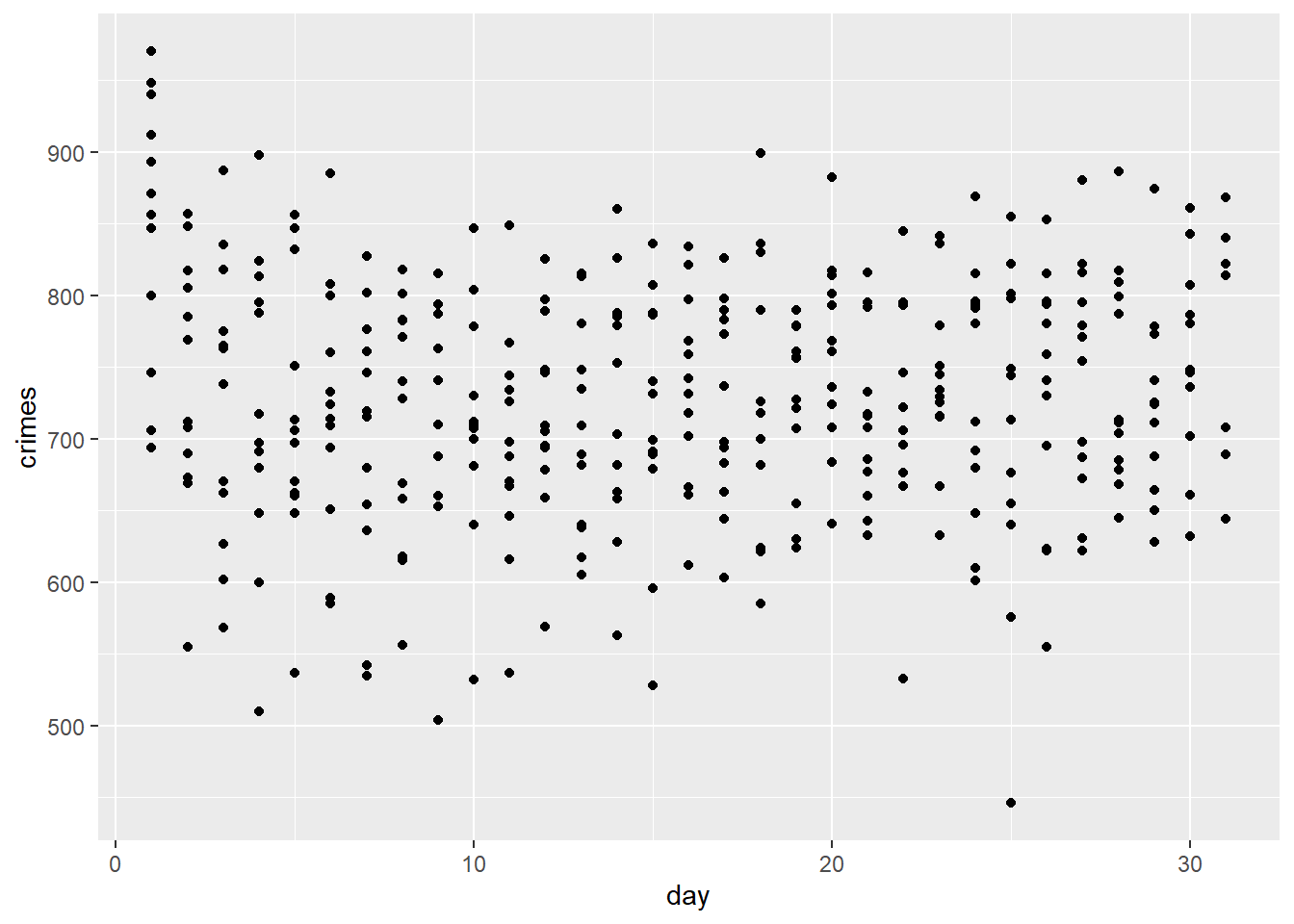
ggplot(temp_data) +aes(x = day, y = crimes) +geom_point()
Wait. This can’t be right. It looks like the day column only runs from 1 up to 31. What’s going on here?
It turns out that the day column in the data just gives the day of the month. How can we plot the data over the course of the entire year?
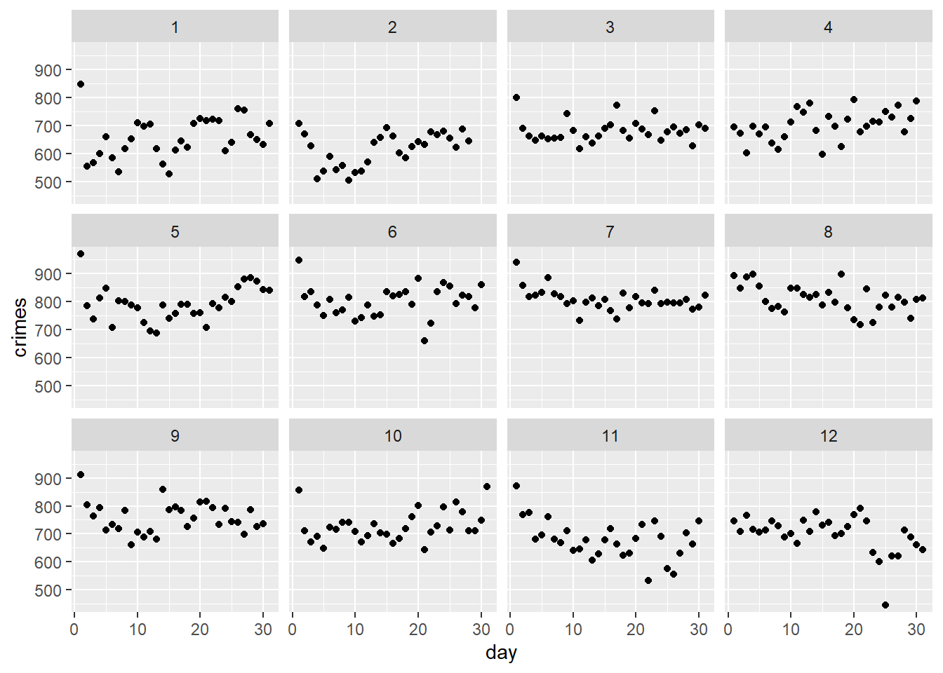
One option is to customize our plot by breaking it down into smaller plots by month. We can do this with the facet_wrap() function:
ggplot(temp_data) +aes(x = day, y = crimes) +geom_point() +facet_wrap(~ month)
That works, but it might also be nice just to have one plot. To do this, we need to create a new day column—one that goes from 1 to 365.
We can modify our data using some other {tidyverse} tools. Let’s use the mutate() function, which lets us mutate or change our data.
temp_data <- temp_data |>mutate(day365 =1:n() )
In the above, I told R I wanted to add a new column to the data called day365 which has values that run from 1 all the way up to the total number of rows in the data (in this case, it should be 365). To check that it worked, I can use the range() function, which will tell me the minimum and maximum values of some vector.
range(temp_data$day365)
[1] 1 365
Looks like it worked. Let’s also just take a quick peak at the data to make sure that the days are in the right order.
ggplot(temp_data) +aes(x = day365, y = crimes) +geom_point()
This is much better.
Really quickly, I want you to notice a few things about ggplot from the code used to produce the above figures. First, ggplot works by building figures in steps. We call these layers. Second, we add layers (literally) by using the + operator. While normally we use this for addition (i.e., 2 + 2) when we use ggplot the + acts a lot like this thing called a pipe operator (%>% or for later versions of R |>). Basically, the + in ggplot just tells R that we want to add a new set of commands or instructions for creating a plot.
More formally, the ggplot workflow looks like:
Feed ggplot data.
Map aesthetics (tell ggplot what relationships to show).
Draw geometry (tell ggplot how to show these relationships).
Customize.
These steps are just a starting point. We can riff on them in various ways to make a more interesting plot. As we do this, another thing to note about making figures with ggplot() is that we can save them as objects in R. Check it out:
p <-ggplot(temp_data) +aes(x = day365, y = crimes) +geom_point()
The object p is our ggplot data viz. Now, every time we write p, it tells R to produce the figure:
p
This feature of working with ggplot is great. The biggest benefit is that it lets us build up a solid foundation for a data viz and then add new details later.
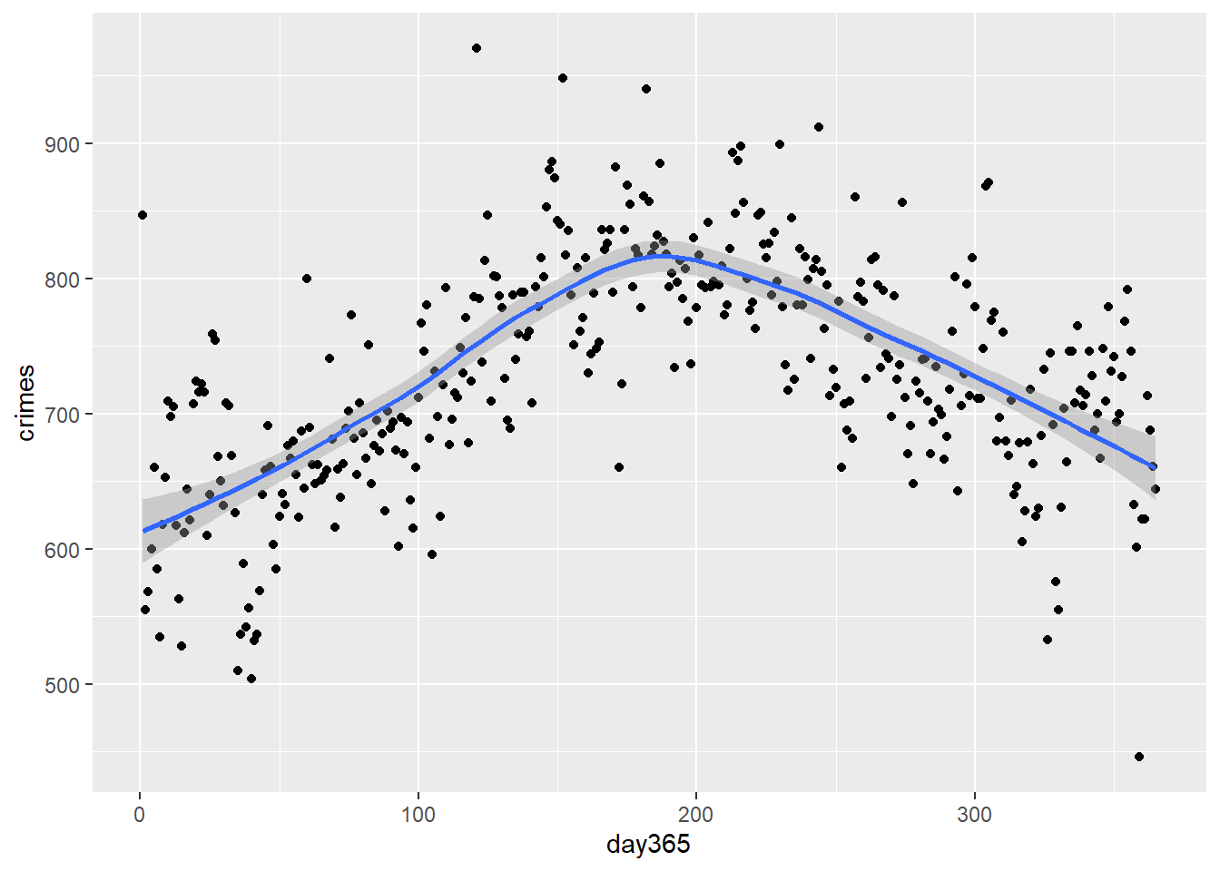
For example, say we want to add another geometry layer, like a regression smoother (basically a model that finds the best fit for the data). All we need to do is add a new layer to p like so:
p +geom_smooth()
`geom_smooth()` using method = 'loess' and formula = 'y ~ x'
Because I saved the first plot as the object p, I didn’t have to re-write the code to produce the old plot before adding a new layer.
In addition to the smoothed model we fit to the data, let’s update the plot labels as well to make them more informative:
p +geom_smooth() +labs(x ="Days",y ="Number of Crimes",title ="Crimes committed in Chicago in 2018" )
`geom_smooth()` using method = 'loess' and formula = 'y ~ x'
The labs() function lets us update the labels of our plot.
3.4 Helpful Resources for Learning More
This class is not about how to use R in its entirety. Here are some resources for you to check out on your own time:
My personal favorite is swirlstats.com, because it lets you work at your own pace directly in R, and for free.
3.5 Wrapping up
Working with code is hard, and I promise you that you will run into problems. When you do, just remember that everyone has problems with their code. It’s normal, and it would be weird if you didn’t have any issues.