9  Reversion to the Mean

9.1 Goals

• Learn about reversion to the mean.
• Understand how people can easily misinterpret data because of reversion to the mean.
• Know when reversion to the mean is and isn’t expected to be relevant.

9.2 The Monty Hall Problem

Have you heard of the show Let’s Make a Deal? Probably not. The show aired decades ago, but it spurred some controversy over a unique probably puzzle the show poses to contestants. Named after the show’s host Monty Hall, this puzzle, dubbed the Monty Hall Problem, has a basic set-up.

A contestant is presented with three closed doors. Behind one is some grand prize, and behind the other two, nothing. The contestant picks a door, blind to what’s behind it. Upon picking the door, Monty Hall would then have one of the other two doors opened. This other door always was one of the doors with nothing behind it. The contestant is then given a choice. Stay with the original door they picked or switch to the other remaining closed door.

What should the contestant do?

If your answer is that it doesn’t matter—she has a 50/50 chance whether she stays or changes—you’d be wrong. In fact, if she changes she’d have a 2/3 probability of winning the prize and only a 1/3 probability of winning the prize if she stays with her original choice.

Confused? Most people are. We human beings have a hard time understanding probabilities. We do much better with certainty. But when we work out the math, this set of probabilities makes logical sense.

Start with the beginning. At the outset, the contestant picks a door. When she does, there is a 1 in 3 chance that her choice is correct. By symmetry, that means there is a 2 in 3 chance that one of the other doors is the correct choice.

Now, when Monty Hall removes one of the other doors, our human intuition leads us to believe that the probabilities have somehow changed. We believe that, now, there is a 1 in 2 chance that the contestant’s choice is right and an equal 1 in 2 chance that the remaining door is the correct choice.

This isn’t true. The probabilities have not, in fact, changed. There are still three doors, but you’re tricked into thinking there are only two when one of the others is opened. There still is a 1 in 3 chance that your original pick is correct and a 2 in 3 chance that your original pick is wrong.

You still may have a hard time believing this. So did the Mythbusters when they tested this out themselves. But it’s actually true.

Here’s a quick simulation to convince you. The below function runs a program that randomly picks a door out of three to put a prize behind. It then has a contestant pick a door at random. Once the contestant picks a door, the program then opens a door that the contestant did not pick and that also does not have the prize behind it. Based on whether change = "no" or change = "yes", the contestant will either keep their original choice or change to the other remaining door. It then returns TRUE if the final choice has the prize behind it or FALSE if otherwise.

monty_hall <- function(change = "no") {
  doors <- as.character(1:3)
  its_here  <- sample(doors, 1)
  pick_door <- sample(doors, 1)
  `%nin%` <- Negate(`%in%`)
  open_door <- sample(doors[doors %nin% c(its_here, pick_door)], 1)
  final_choice <- ifelse(
    change == "no", pick_door, doors[doors %nin% c(pick_door, open_door)]
  )
  final_choice == its_here # returns TRUE if yes
}

I then replicate the game 4,000 times. In 2,000 of those times the contestant always changes their door choice. In the remaining 2,000 she stays with original choice.

## open {tidyverse} 
library(tidyverse)

## simulate outcomes and save in object called "outcomes"
tibble(
  it = 1:4000,
  choice = rep(c("yes", "no"), each = max(it) / 2),
  outcome = map2(
    .x = it,
    .y = choice,
    .f = ~ monty_hall(.y)
  ) |> unlist()
) -> outcomes

Let’s check how the contestant did by switching relative to keeping with her original choice:

outcomes |>
  group_by(choice) |>
  summarize(
    win_rate = mean(outcome),
    std_error = sd(outcome) / sqrt(n()),
    lo = win_rate - 1.96 * std_error,
    hi = win_rate + 1.96 * std_error
  ) |>
  ggplot() +
  aes(x = choice, y = win_rate, ymin = lo, ymax = hi) +
  geom_col(width = 0.5) +
  geom_errorbar(width = 0.25) +
  scale_y_continuous(
    breaks = c(1/3, 2/3),
    labels = c("1/3", "2/3")
  ) +
  labs(
    x = "Change door?",
    y = "Win rate",
    title = "The Monty Hall Puzzle in Action"
  )

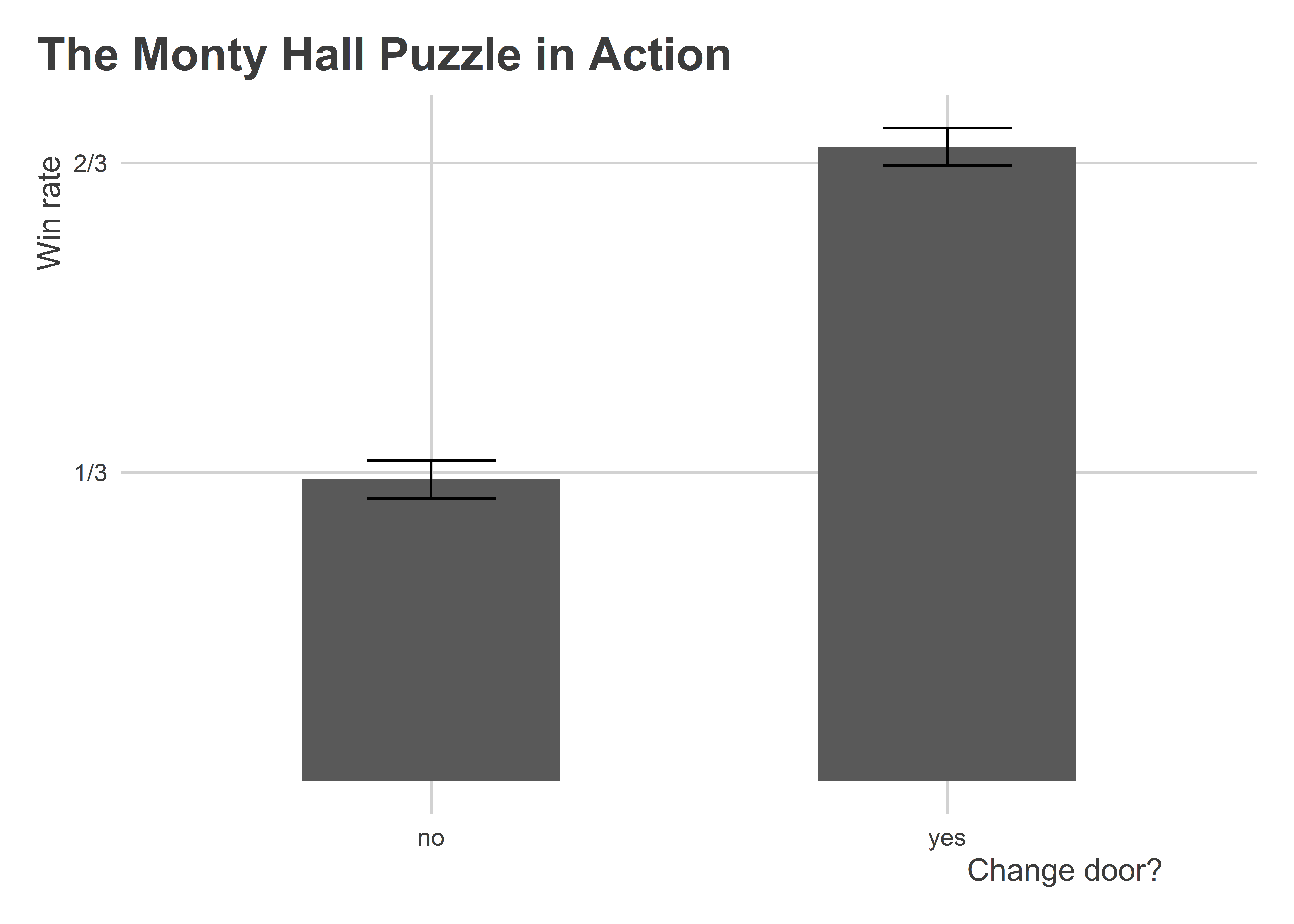
Remarkably, switching is the superior choice! This actually shouldn’t be that surprising, but no matter how many times I run this simulation, I have a hard time wrapping my brain around the probabilities. But the numbers don’t lie. And if you’re thinking that simulation is broken, it isn’t. I’ve checked.

Now, you probably are thinking to yourself, what does any of this have to do with reversion to the mean? It turns out that the probability puzzle that makes the Monty Hall Problem so mind-bending is the same kind of probability problem that explains reversion to the mean.

9.3 What is reversion to the mean?

Let’s look at some 2016 election data for the state of Ohio. This dataset provides county-level detail on how people voted in the 2016 election for President, in addition to how people voted in 2012.

Data <- socviz::county_data |>
  filter(state == "OH") |>
  drop_na()

We can make a scatter plot just like John Galton’s for heights between parents and their children which Bueno de Mesquita and Fowler (2021) discuss in their book. We’ll do this using demeaned election margins for the GOP Presidential candidate in 2012 on the x-axis and demeaned election margins for the GOP Presidential candidate in 2016 on the y-axis. For each, just like with Galton’s height data, we’ll rescale the data to standard deviation units around the mean, too.

## make function to "demean" a variable
demean <- function(x) (x - mean(x, na.rm=T)) / sd(x, na.rm = T)

## visualize
ggplot(Data) +
  aes(x = demean(per_gop_2012),
      y = demean(per_gop_2016)) +
  geom_point() +
  geom_smooth(
    method = lm,
    se = F
  ) +
  geom_abline(
    slope = 1, 
    intercept = 0,
    lty = 2
  ) +
  labs(
    x = "Demeaned margin for GOP in 2012",
    y = "Demeaned margin for GOP in 2016",
    title = "Reversion to the mean in Ohio, 2012-2016",
    caption = "Data: {socviz}"
  )

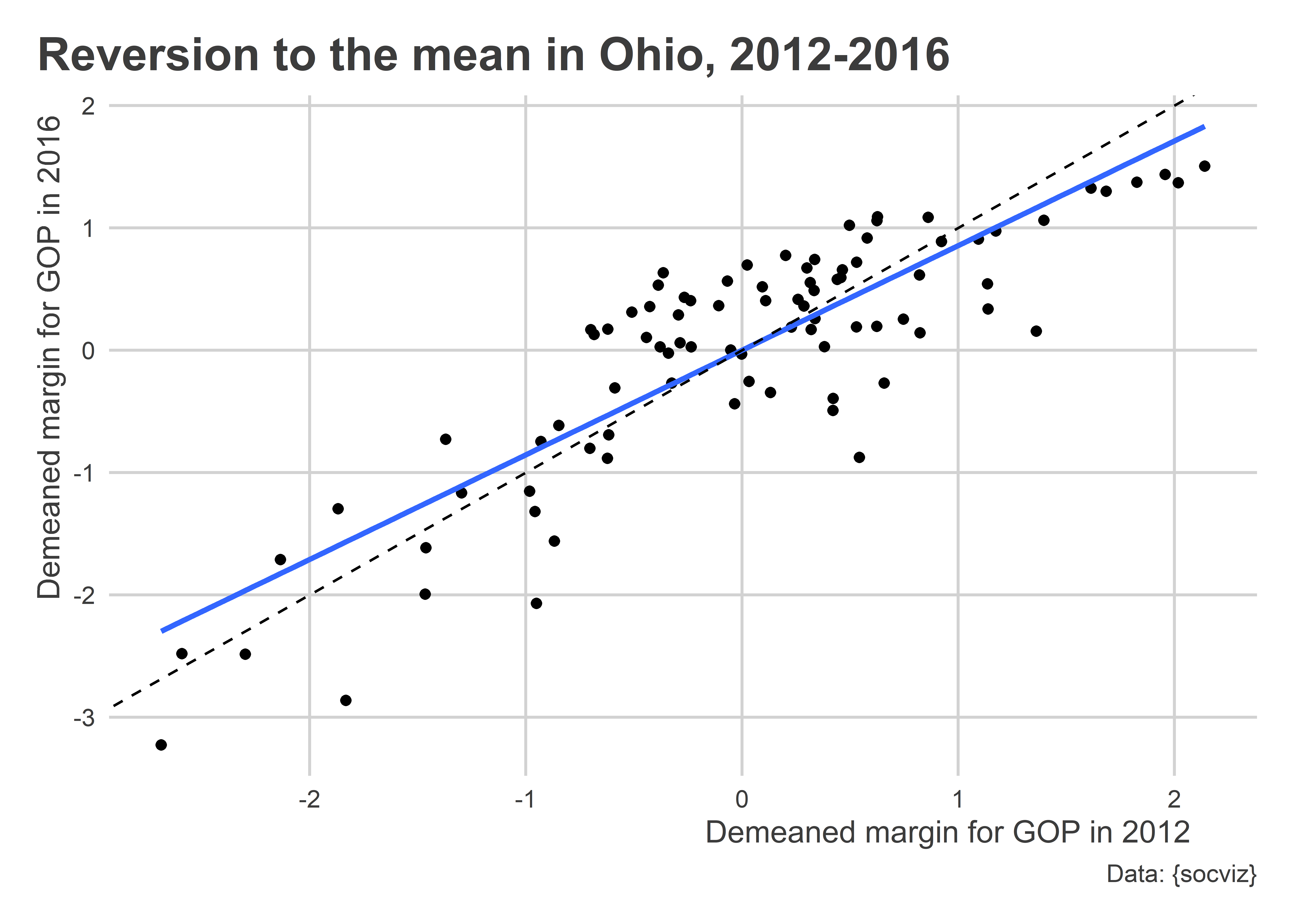
The above figure clearly shows evidence of reversion to the mean. The trend is modest, but it is there. Intuition would lead us to believe that there should, on average, be a 1-to-1 correspondence between how well the GOP did in 2012 to how well it did in 2016. In reality, in places where the GOP did especially poorly in 2012 they did better in 2016. Conversely, in places where the GOP did especially well in 2012, they did slightly worse in 2016.

This pattern of reversion to the mean is common to many phenomena, and it is often why many analysts and commentators make erroneous inferences from one election cycle to the next. As Bueno de Mesquita and Fowler (2021) remind us time and again, our estimates with data reflect not just signals but also noise and bias. That means outcomes in elections can shift from one to the next, not just because of changes in the mood of the electorate but also because of random and systemic unobserved factors (signal + noise).

Especially extreme observations can be the product of signal, but also a good deal of noise. For that reason, it would be unsurprising to see future outcomes revert to the overall mean of the factor in question.

This happens for the same reason that switching your choice in Let’s Make a Deal gives you a better chance of winning the grand prize. Consider the normal distribution. Say we have a variable x that is normally distributed with mean of zero and standard deviation of 1. The below figure summarizes the probabilities of seeing different values of x:

Say that we take a random draw from this distribution and get x = -1.5. If we took another random draw from the distribution, do you think it will be smaller or bigger than this value?

Theoretically, there’s a good chance that it will be bigger. To put a precise probability on it, there would be a 93.32% chance of observing some value of x greater than -1.5. Check it out:

Now, imagine that we draw another number, but before I reveal it to you I told you than it is definitely not equal to 0. Would this change you calculation? It shouldn’t for the same reason that it shouldn’t in the Monty Hall Problem. If we observe an extreme value, there’s always a good chance that the next one we observe will be less extreme.

9.4 Try it out

Adapt the following code to pick a state of your choosing and make a plot like the one I produced for Ohio. Do you see evidence of reversion to the mean?

# Make the demean function
demean <- function(x) x - mean(x, na.rm=T)

# Pick your state
my_state <- "OH" # I picked Ohio, but you can pick any

# Get your data
Data <- socviz::county_data |>
  filter(state == my_state) |>
  drop_na()

To check whether there is reversion to the mean, you can also estimate a simple linear regression. If the slope is less than 1, that would be consistent with reversion to the mean. Can you think of a way to devise a hypothesis test where the null is that the slope is equal to 1?

Bueno de Mesquita, Ethan, and Anthony Fowler. 2021. Thinking Clearly with Data: A Guide to Quantitative Reasoning and Analysis. Princeton University Press.