Understand what a hypothesis is and how we test them using statistics.
Understand what a p-value is (and isn’t).
Understand that we never accept hypotheses. We can only reject or fail to reject them.
Know how to calculate the right kinds of standard errors to properly test against the null hypothesis.
Consider why over-comparing and under-reporting of research findings is bad for the general accumulation of scientific knowledge.
8.2 What is a hypothesis and how do we test it?
When we test a hypothesis in science we usually are dealing with two hypotheses simultaneously. We call these the null hypothesis and the alternative hypothesis.
The null hypothesis is usually a statement about theequality between two things. It could be that the mean of x in group A is equal to the mean of x in group B. Or it could stipulate that the correlation between x and y is equal to zero. Whatever it is, it takes the form of something being equal to something else. This statement about the equality of two (or more) things is called the null hypothesis because it states that we expect to see a null relationship or estimate with our data.
The alternative hypothesis is a proposition, usually informed by a theoretical argument, about some non-zero estimate or relationship we expect to see in the world. For example, Democratic Peace Theory argues that democratic countries are unlikely to go to war with each other because they share common values and have a system of governance based on negotiation and compromise. A hypothesis that follows from this is that we should expect to see lower rates of conflict, or less intense conflict, between pairs of democracies than between other kinds of countries.
These two hypotheses form the basis for formal hypothesis testing using statistics, but they serve different functions. The null hypothesis serves as a point of reference and it is the actual hypothesis that we test using statistics. Specifically, using the null hypothesis as our starting point, we use statistics to calculate the probability that we would get the estimate we calculated with our data if the null hypothesis were true. This probability is called the p-value, and a good way to think of it is as a summary of how embarrassed the null hypothesis is by our data. A very small p-value means there is very little evidence in the data to support the null—pretty embarrassing.
The alternative hypothesis, even though we don’t formally test it with statistics, is still important because it is our rationale for conducting a hypothesis test in the first place. Say we test the null hypothesis analogue to our alternative hypothesis about the Democratic Peace. Why would we want to test whether rates of conflict between pairs of democracies are the same as between other kinds of countries (the null hypothesis)? The motivation is the fact that theory tells us we should see something contrary to the null hypothesis.
As we test against the null hypothesis, it is important to be precise in the language we use to describe the results of our hypothesis test. A foundational principal of scientific inquiry is the falsificationprincipal. In science, we can never prove a proposition to be true using empirical evidence because it is always possible that some future data or test will give us different results. The best we can do is to falsify a hypothesis or fail to falsify it. For this reason, when we test against the null hypothesis we can only either reject the null hypothesis on the basis of the data or fail to reject it. We never accept a hypothesis. For example, if we can reject the null hypothesis, that does not imply that we should accept the alternative.
8.3 We use p-value thresholds to reject or fail to reject the null
We use p-values to determine whether we can reject or fail to reject the null. The traditional practice is to use a pre-determined p-value threshold as our basis for rejecting the null. This threshold is called the level of the test and we usually represent this value as \(\alpha\) or the \(\alpha\)-level and we say that we can reject the null if the p-value is less than this value. The convention is to set \(\alpha = 0.05\). This is admittedly arbitrary, and whether this is an appropriate threshold is the subject of much debate. Nonetheless it remains the default for most quantitative researchers.
8.4 We use standard errors to help us calculate the p-value
Since a p-value is a probability we need some criterion for calculating it based on the results we get with our data. In a regression analysis with the OLS estimator, we use a t-statistic associated with our observed regression estimates to get p-values. This statistic has a known theoretical distribution where different values in this distribution have different probabilities of occurring by random chance depending on how many observations we have in our data.
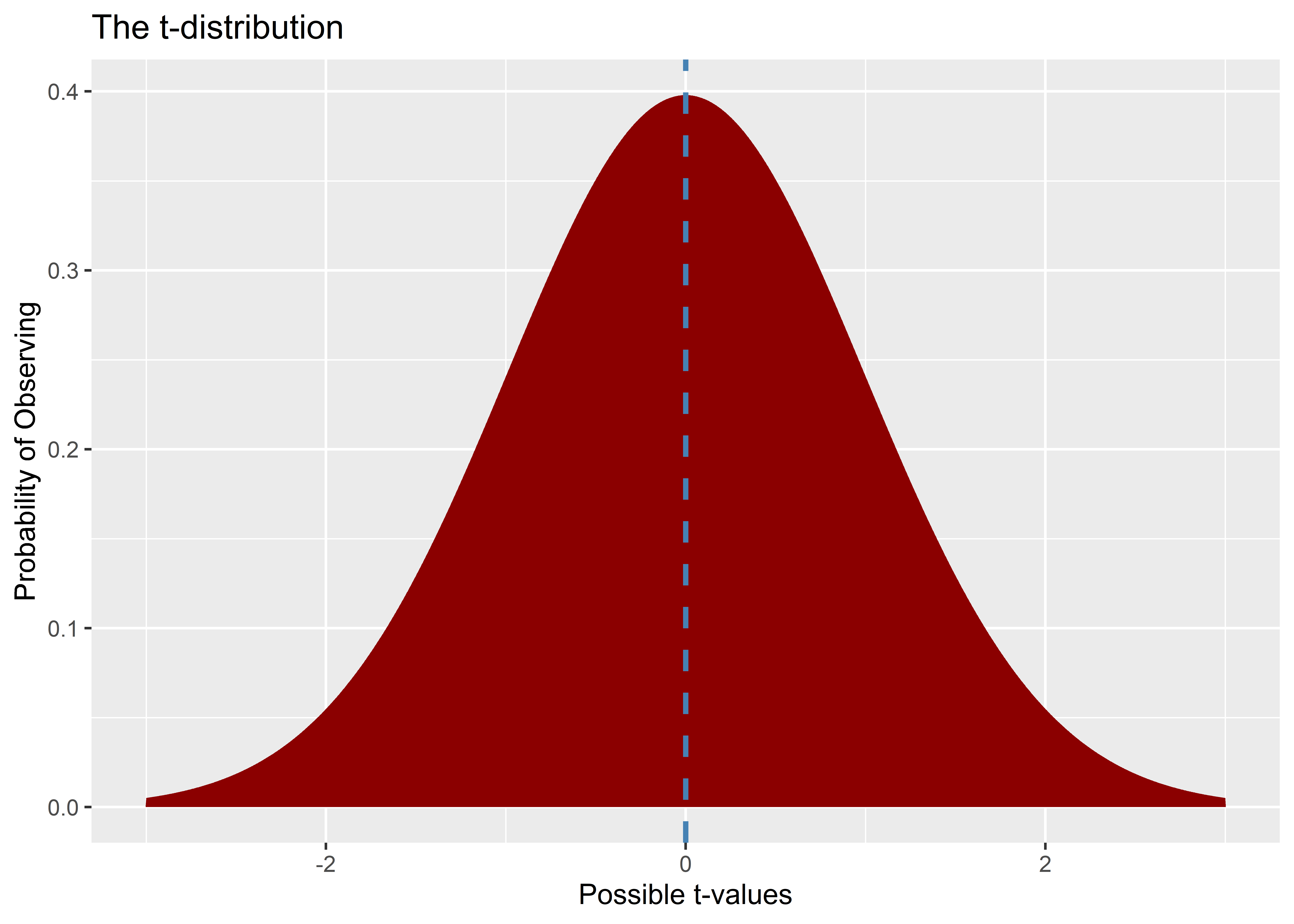
The below R code visualizes a t-distribution for data with 100 observations. Notice that it looks a lot like a normal distribution (however if you compared it to a normal distribution you’d notice that the t-distribution is a bit thicker in its tails). It has a central tendency (mean) of zero and symmetrical variation around that central tendency with values farther from zero expected to occur with lower frequency.
## tell R to draw a t-distributiontibble(x =seq(-3, 3, by =0.01),t =dt(x, df =100)) |>ggplot() +aes(x = x, y = t) +geom_area(fill ="red4" ) +geom_vline(xintercept =0,linetype =2,size =1,color ="steelblue" ) +labs(x ="Possible t-values",y ="Probability of Observing",title ="The t-distribution" )
Since we have a known theoretical distribution associated with different t-values, all we need to do is calculate a t-value for the estimate we get with our data. Our software will then take care of the process of cross-referencing this t-value with the right distribution to give us the p-value. Of course, this begs the question: how do we calculate the t-value?
In the last chapter we discussed using standard errors for statistical inference. Standard errors are also essential in hypothesis testing because we need them to calculate the t-value for our estimate. Say we estimate a regression model and get a slope coefficient of \(\hat \beta_1\) and a standard error of \(\sigma_\beta\). The t-value for this estimate is just the ratio of the slope to its standard error:
\[
t = \frac{\hat \beta_1}{\sigma_\beta}
\]
With a t-value calculated, we can then use its associated p-value to determine if we should reject the null hypothesis for our particular estimate based on our selected \(\alpha\)-level for the test.
8.5 An example in R
Let’s look at some data on international conflicts to illustrate the process of hypothesis testing. The below code will open the {tidyverse} and read in a conflict series dataset that documents 1,550 unique militarized interstate confrontations (MICs) that have taken place between countries from 1816 to 2014. A MIC is anything from a show or threat to use military force by one country against another up to and including all-out war.
## open {tidyverse}library(tidyverse)## read in the dataurl <-"https://raw.githubusercontent.com/milesdwilliams15/Teaching/main/DPR%20201/Data/mic_data.csv"Data <-read_csv(url)
For each confrontation in the data there are a number of variables we can examine such as the number of fatalities by confrontation’s end, when the confrontation started and how long it lasted, and some information about the countries involved. Say, based on Democratic Peace Theory, we want to test whether confrontations among more democratic countries are less intense than those among less democratic countries. Using our data, one way to test this proposition is using conflict fatality data and a measure of the average democracy scores among the countries involved in a confrontation. Based on our theory, the alternative hypothesis would be stated as follows:
H(A): Confrontations among countries with higher average democracy scores will end in fewer fatalities.
The null hypothesis analogue to this hypothesis that we will actually test with the data is then:
H(0): Confrontations among countries with higher average democracy scores will end in the same number of fatalities as confrontations among countries with lower average democracy scores.
To test this hypothesis we’ll use a simple linear regression model that we estimate using OLS. Specifically:
The next step is to use the summary() function on model_fit. This function lets us perform statistical inference on the regression model parameters. It will report standard errors for the slope and intercept in addition to their t-values and p-values.
summary(model_fit)
Call:
lm(formula = fatalmax ~ mean_democracy, data = Data)

Residuals:
     Min       1Q   Median       3Q      Max
  -43529   -25276   -19624   -15170 15468035

Coefficients:
               Estimate Std. Error t value Pr(>|t|)
(Intercept)       22768      12828   1.775   0.0761 .
mean_democracy   -12638      21055  -0.600   0.5484
---
Signif. codes:  0 '***' 0.001 '**' 0.01 '*' 0.05 '.' 0.1 ' ' 1

Residual standard error: 480700 on 1548 degrees of freedom
Multiple R-squared:  0.0002327, Adjusted R-squared:  -0.0004131
F-statistic: 0.3603 on 1 and 1548 DF,  p-value: 0.5484
The the values under Pr(>|t|) are p-values. As you can see, the p-value for the slope on mean_democracy is 0.5484. This is the probability, if the null hypothesis is true, of seeing the t-value of -0.6 calculated for mean_democracy by random chance. Based on the results, we’d expect to see this estimated t-value over 50% of the time if the null were true by dumb luck alone. Since, by convention, we use a p-value of 0.05 or less as our threshold for rejecting the null hypothesis, in the above example we can’t reject the null. While we observe a negative coefficient on the democracy measure, its value is not all that unlikely to have arisen by random chance.
8.6 Make sure your inferences are robust
At this point in our discussion about hypothesis testing and inference, it bears noting that our calculations of standard errors involve equations that make some strong assumptions. These assumptions often are not justified or are unlikely for many kinds of data. For this reason, you should always calculate robust standard errors. These are calculated using equations that impose weaker assumptions about our data.
The main assumptions that we need to be worried about when it comes to inferences with an OLS regression are:
That model errors are independently distributed (there is no clustering)
That model errors are identically distributed (there is no heteroskedasticity)
Independently and identically distributed (iid) errors are essential for the classic standard errors calculated with the summary() function in R to be valid. For errors to be independently distributed, it must be the case that outcomes for one observation in the data aren’t correlated or determined by outcomes for other observations in the data. For errors to be identically distributed, it must be the case that an observation’s outcome is not somehow related to the size of its error (its expected value from the model and its actual value).
The first kind of problem can be solved by using a standard error that allows for clustering, and the second can be solved by using a standard error that is robust to heteroskedasticity. Thankfully, we can calculate both kinds of standard errors in R.
One way we can calculate them is with by bootstrapping. A strength of bootstrapping as a default approach to inference is that it lets us make inferences on the basis of our data itself rather than some theoretical assumptions about our data that may or may not hold up.
There are many ways to go about bootstrapping a regression model in R. Here’s some code I put together to make it happen. I begin by creating a function called boot_summary() which works a lot like the standard summary() function, but it reports bootstrapped inferences instead of classical inferences:
boot_summary <-function(model, its =200) {## get model data model_data <-model.frame(model)## get model formula model_formula <- model_fit$call[[2]]## bootstrap the model and return a summary tabletibble(it =1:its,boot_est =map( it, ~ {lm( model_formula,data = model_data |>sample_n(size =n(), replace = T) ) -> boot_fittibble(term =names(coef(boot_fit)),estimates =coef(boot_fit) ) } ) ) |>unnest( boot_est ) |>group_by( term ) |>summarize(std_error =sd(estimates) ) |>ungroup() |>mutate(estimate =coef(model),t_value = estimate / std_error,p_value =2*pt(-abs(t_value), df = model$df.residual) ) |>select(term, estimate, std_error, everything())}
With this new function, we can check out how our inferences differ with bootstrapping:
It turns out that the standard errors with summary() might have been too pessimistic. The p-value above still isn’t below the threshold of 0.05, but it’s much closer.
If we wanted to allow for clustering, instead of bootstrapping individual observations we’d bootstrap groups. We could easily make an updated boot_summary() function that performs a clustered bootstrap if we wanted. However, there are already some simpler approaches at our disposal in R.
Another way we can make robust inferences with R is to use tools from the {sandwich} and {lmtest} packages. The below code uses coeftest() from {lmtest} in combination with vcovHC() from {sandwich} to report a kind of robust standard error called HC1 standard errors. Generally speaking, these are the recommended robust standard errors for linear regression models (when we discuss causal inference in the next part of this book, we’ll introduce a different kind of robust standard error). As you can tell from the output, the results are pretty similar to what we got using bootstrapping.
## open {sandwich} and {lmtest}library(sandwich)library(lmtest)## use coeftest() and vcovHC()coeftest( model_fit,vcov. =vcovHC(model_fit, type ="HC1"))
t test of coefficients:

               Estimate Std. Error t value Pr(>|t|)
(Intercept)     22768.1    13493.1  1.6874  0.09173 .
mean_democracy -12638.4     7014.9 -1.8017  0.07179 .
---
Signif. codes:  0 '***' 0.001 '**' 0.01 '*' 0.05 '.' 0.1 ' ' 1
The nice thing about this approach to robust inference is that the {sandwich} package includes functions that will perform clustered inference as well. Say, for example, we were concerned that militarized confrontations in our data that start in the same year are somehow related to each other and we’re concerned that this violates the independence assumption of our standard errors. We can replace the vcovHC() function with the vcovCL() function and specify that we want to cluster on year. Interestingly, our standard errors are smaller when we cluster on year, meaning our p-value is even closer to the 0.05 threshold.
## use vcovCL() instead of vcovHC()coeftest( model_fit,vcov. =vcovCL(model_fit, cluster = Data$year, type ="HC1"))
t test of coefficients:

               Estimate Std. Error t value Pr(>|t|)
(Intercept)     22768.1    13419.6  1.6966  0.08997 .
mean_democracy -12638.4     6910.9 -1.8288  0.06763 .
---
Signif. codes:  0 '***' 0.001 '**' 0.01 '*' 0.05 '.' 0.1 ' ' 1
A third way (and my favorite way) to make robust inferences with a linear model is to use the lm_robust() function from the {estimatr} package in place of the base R lm() function. lm_robust() works just like lm() except it has an option to control what kind of standard errors it should report for the model coefficients. By setting se_type = "HC1" the function reports the appropriate HC1 standard errors. As you can see from the output, by default lm_robust() provides inferences without the need to use a summary() function. It also gives us 95% confidence intervals which we don’t get using the base R summary() function or by using coeftest().
## open {estimatr}library(estimatr)## use lm_robust()lm_robust( fatalmax ~ mean_democracy,data = Data,se_type ="HC1")
                Estimate Std. Error   t value   Pr(>|t|)   CI Lower  CI Upper
(Intercept)     22768.08  13493.113  1.687385 0.09173079  -3698.631 49234.786
mean_democracy -12638.44   7014.853 -1.801669 0.07179200 -26398.062  1121.175
                 DF
(Intercept)    1548
mean_democracy 1548
If we want output that looks closer to summary() for lm(), there’s a version of the summary() function that works with lm_robust(). Here’s what the output looks like:
Call:
lm_robust(formula = fatalmax ~ mean_democracy, data = Data, se_type = "HC1")

Standard error type:  HC1

Coefficients:
               Estimate Std. Error t value Pr(>|t|) CI Lower CI Upper   DF
(Intercept)       22768      13493   1.687  0.09173    -3699    49235 1548
mean_democracy   -12638       7015  -1.802  0.07179   -26398     1121 1548

Multiple R-squared:  0.0002327 ,    Adjusted R-squared:  -0.0004131
F-statistic: 3.246 on 1 and 1548 DF,  p-value: 0.07179
We can also adjust for clustering with lm_robust() using the clusters option. Notice that when we want to report clustered robust standard errors we also need to set se_type = "stata". If you compare the output to what we got using vcovCL() with {sandwich} you’ll notice that the inferences are the same.
lm_robust( fatalmax ~ mean_democracy, data = Data,se_type ="stata",clusters = year)
                Estimate Std. Error   t value   Pr(>|t|)   CI Lower   CI Upper
(Intercept)     22768.08  13419.564  1.696633 0.09145703  -3707.923 49244.0784
mean_democracy -12638.44   6910.882 -1.828774 0.06905237 -26273.203   996.3156
                DF
(Intercept)    184
mean_democracy 184
8.7 Avoid over-comparing and under-reporting
As you conduct statistical analyses, you’ll quickly realize that how you choose to measure a variable, what variables you choose to include in a regression model, and how you choose what observations to include in your analysis will change your results. It won’t be long after this realization that you’re tempted to taste the forbidden fruit of p-hacking.
P-hacking is the act of torturing data until it confesses, and it has become an important problem in scientific research. The problem with using torture to elicit a confession is that the one being tortured will say anything to make the suffering stop, no matter if the confession is true or a false. The same is true with data. If you torture a dataset long enough it will eventually tell you what you want it to say, but that doesn’t mean that what it says is true.
P-hacking is done by performing any number of data transformations or alternative regression model specifications until a non-significant result becomes significant. FiveThirtyEight published a p-hacking dashboard to illustrate how this process can work. I highly recommend checking it out, because it shows how seemingly trivial choices about your data or statistical model can amount to massive swings in the magnitude and statistical significance of estimates.
To the extent that this practice is widespread, it harms the accumulation of scientific knowledge, especially if researchers aren’t transparent about the choices they made in performing an analysis. A researcher could have tried 20 different approaches in their analysis only to report the results from the 1 out of 20 that gave them the result they were looking for. If enough researchers do this, then the sum total of scientific research is biased in favor of finding statistically significant and large estimates than would be supported by a more representative sample of research. As we move on to talking about causation, we’ll discuss some strategies for minimizing this practice, such as pre-registration of analysis plans prior to seeing data. Another strategy is to crowd-source research by recruiting multiple research teams to answer a research question rather than relying on one team or even just one individual doing the research. Such approaches help to illuminate researcher degrees of freedom, or the extent to which researcher choices can influence the range of results you can get out of a dataset.
Short of the above approaches, one increasingly popular antidote to p-hacking is open science—the idea of making all data and code used to analyze it publicly available. This gives others an opportunity to validate and question the findings published by others, which hopefully serves to catch any possible instances of p-hacking if another researcher discovers that the findings published by someone else are highly sensitive to analysis choices.
Ultimately, it’s your responsibility to make ethically sound and transparent choices in your analysis. P-hacking is easy to identify in a body of research, but it’s difficult to say that it occurred in a particular study. It’s sometimes quite easy to disappear in a crowd. So be careful and be mindful of your actions.
8.8 Conclusion
Hypothesis testing is a central part of scientific inquiry, so it is important to understand how we go about it when doing quantitative research. Hypothesis testing provides a rigorous means to quantifying uncertainty and summarizing the extent to which our data is consistent with what we expect to see.
Importantly, when we test hypotheses we do so with two hypotheses in mind: a null hypothesis and an alternative hypothesis. The latter is a theoretically motivated prediction of what we should expect to see in the world which motivates our research, while the former is what we actually put to the test and try to reject using statistics.
To test against the null hypothesis, we calculate a p-value, which is the probability of getting an estimate that we observe with our data by random chance if the null hypothesis is true. We use an \(\alpha\)-level or level of the test as a p-value threshold to determine whether we can reject or fail to be able to reject the null hypothesis. Importantly, we never accept hypotheses in scientific research, nor do we prove a hypothesis is true.
To calculate p-values we need to perform statistical inference, which means we need to compute standard errors for our estimates. We then can use the ratio of our estimate to its standard error to calculate a t-value which we compare to a theoretical distribution to figure out its probability of occurring by random chance under the null.
As we perform hypothesis testing, it is important to ensure that we use the most appropriate standard errors. By default, we should use robust standard errors, and if we suspect that there is clustering in our data we should calculate robust clustered standard errors instead. This will ensure that our inferences actually reflect the variation in our data rather than a theoretical distribution that doesn’t fit.
It finally is important to ensure that we are ethical in our approach to hypothesis testing and avoid p-hacking. We all want to find statistically significant results, but if we have to torture our data to get what we want it’s possible that our results will only mislead rather than illuminate. Be vigilant and find ways to keep yourself accountable.