library(tidyverse)
library(socsci)
library(estimatr)
library(texreg)
library(coolorrr)
set_theme()
set_palette(
  binary = c("gray", "black")
)14 Regression Discontinuity Designs
14.1 Goals
- Controlling for covariates in a selection on observables or SOO design using a multiple regression model is one way to recover causal estimates from non-experiments.
- But SOO designs are notoriously susceptible to omitted variable bias and a host of other challenges.
- However, in some settings we can exploit certain facts about how data were generated to make more reliable causal inferences.
- One such approach is to use a discontinuity in some data to estimate a local average treatment effect or LATE.
- When we do this, we are using a regression discontinuity design or RDD.
Packages you need:
14.2 What is a regression discontinuity design?
A regression discontinuity design or RDD is a kind of research design known as a quasi-experimental design (QED). QEDs are a class of research designs where we can leverage sources of random variation in how a treatment or causal variable was assigned to estimate its causal effect on an outcome. We aren’t dealing with a true experiment, however. Hence the quasi modifier on QEDs.
Importantly, in many QEDs, including RDDs, since we need to find a way to turn a non-experiment into an experiment, we’re forced to narrow our causal inferences in some way—to localize them to observations in the data where treatment assignment really is random. For this reason, the estimator we use in QEDs is not the usual average treatment effect or ATE that we would calculate in a randomized controlled trial (RCT). Rather, we use a variation on the ATE known as the local average treatment effect or LATE. The idea is that our estimate of the ATE is local to observations where assignment of the causal variable is plausibly random.
RDDs are a powerful tool for recovering an estimate of the LATE. They work by leveraging some discontinuity or threshold in our data where the differences between observations that get “treated” and those that don’t are (hopefully) unrelated to both the outcome of interest and the treatment variable.
To implement an RDD to answer a causal question, we need just a few basic things in our data:
- An outcome
- A treatment (usually this is binary)
- A (semi-)continuous running variable that determines treatment assignment
Our tool of choice for implementing RDDs is the same as our preferred tool for controlling for confounders in an SOO design: multiple regression. But, while the tool is the same, how we specify our linear model and interpret the results will be different because of what we know about the data-generating process.
What we generally want to do is estimate the effect of the treatment right at the point of some relevant discontinuity or threshold in the data. To do that, we need to use an interaction between a treatment indicator and a factor called the running variable. This running variable is related to treatment assignment in that it defines a threshold or point of discontinuity defining when or where treatment is assigned. Ideally our running variable will be set so it equals zero precisely at the point of this discontinuity.
Consider some U.S. House incumbency data that we can access in R using the package {rddtools}. This data comes from a paper published by Lee (2008) to test whether U.S. House members enjoy an incumbency advantage—this is an extra electoral boost members of congress get simply because they are running for reelection rather than for the first time. To access the data, you’ll need to install {rddtools}. Then you can write:
library(rddtools)
data(house) #Lee data
head(house)
x y
1 0.1049 0.5810
2 0.1393 0.4611
3 -0.0736 0.5434
4 0.0868 0.5846
5 0.3994 0.5803
6 0.1681 0.6244The dataset has two columns, x and y, that correspond to the Democratic vote margin in year t (column x) and the Democratic vote share in year t+2 (column y). If x < 0, then a candidate lost the previous election. If x >= 0, then a candidate won the last election and, hence, is an incumbent.
We have all the building blocks we need to implement an RDD. But first we should probably discuss why we need an RDD to test the incumbency advantage in the first place.
The big question you should ask yourself is whether being an incumbent is correlated with other factors that might give a candidate an electoral boost? The answer is probably yes. Perhaps a candidate is uniquely popular, or maybe a congressional district is a historical stronghold for a particular party. Both of these factors would explain why a particular candidate won in a previous election and also why they can expect to win in the next. This fact should lead us to be cautious in our approach to estimating an incumbency advantage because both of these factors explain why a candidate is an incumbent and why they can expect to win in the next election. Basically, our raw estimate of the effect of being an incumbent is probably going to be subject to omitted variable bias.
However, there are always little random differences from one election to the next. The weather could be better in one election versus the previous. Different issues may be salient. A scandal could have surfaced. Anything! The beauty of RDD is that it gives us a way to leverage all these little sources of random variation to get around omitted variable bias. This works by identifying the precise threshold needed for an observation to be “treated” with incumbency. That is precisely the point between winning an election with a majority of the vote, or just failing to reach this threshold. By estimating the effect of incumbency locally among close elections, we can get a reliable estimate of incumbency’s causal effect on future election performance.
To see how we can force our estimate to be local to these close elections, let’s look at the anatomy of a RDD regression model specification with the U.S. House data. Here’s the model we need to estimate:
\[ \text{Vote Share}_{it+2} = \beta_0 + \beta_1 \text{Incumbent}_{it} + \beta_2 \text{Vote Margin}_{it} + \beta_3 \left(\text{Incumbent}_{it} \times \text{Vote Margin}_{it} \right) + \epsilon_{it+2} \]
The outcome variable here is the vote share for the Democratic Party in a future election. The predictor variables in the model include a binary indicator for whether the Democratic Party is the incumbent party (the causal variable of interest) and a continuous measure of the Democratic Party’s vote margin in the previous election. Notice that both of these variables make independent appearances in the model and also a combined appearance as an interaction term. This extra term imbues the estimate on incumbency with a very special, conditional interpretation. Rather than this estimate being equivalent to an average overall difference in expected vote share due to incumbency, it is the expected difference in vote share exactly at the point where the vote margin is zero. The average difference, in short, is local to the majority threshold required for a candidate to win in a previous election and, hence, to be an incumbent in the next.
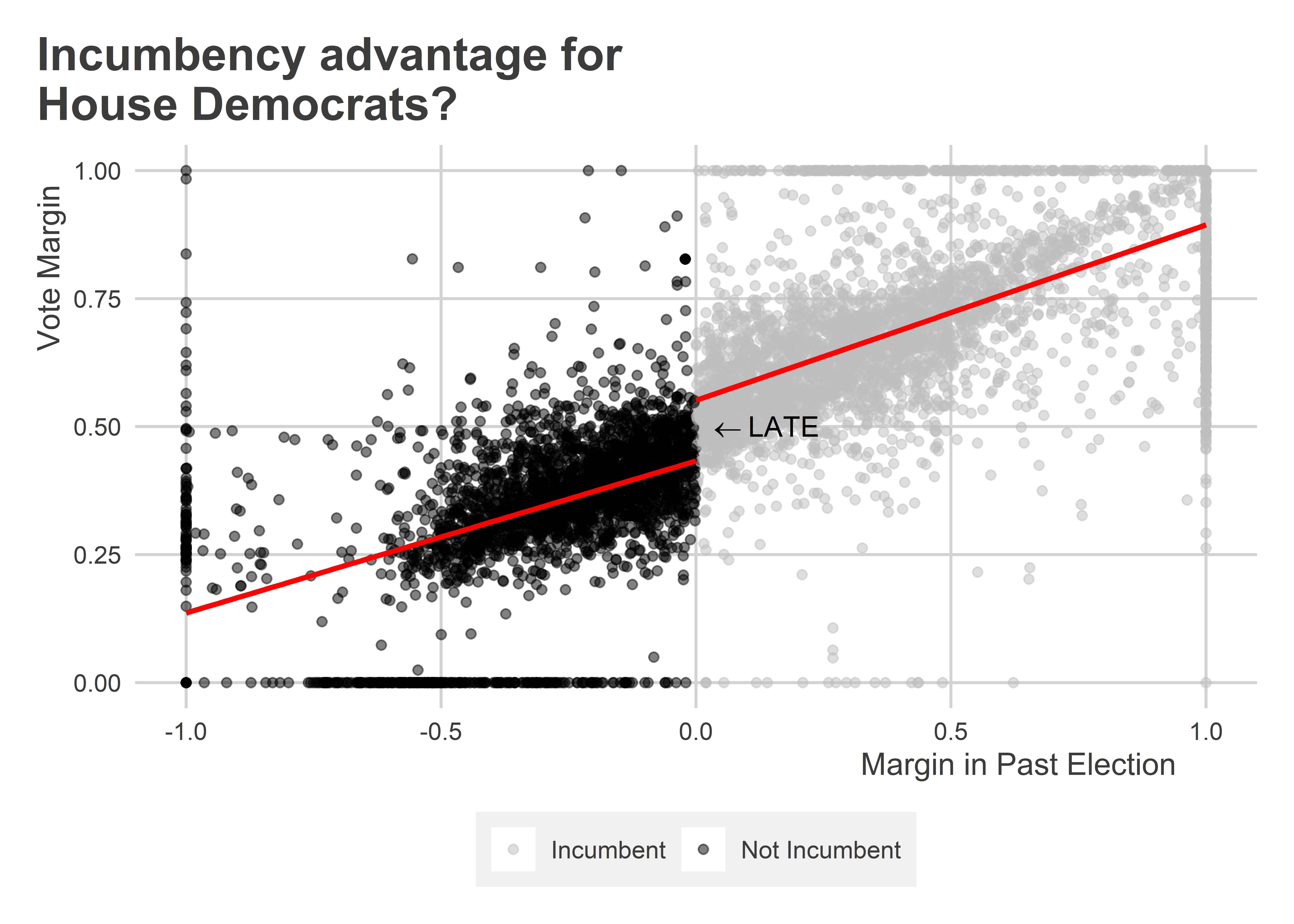
The idea may be clearer by visualizing the data. The above regression model gives us this local estimate by leting us estimate two different regression slopes with different intercepts per the incumbency cutoff in the data. Check out the below visualization. It shows the vote margin for the Democratic Party on the x-axis in the previous congressional election per congressional district. It shows the vote margin for the Democratic Party on the y-axis for the next election year. If the previous election’s margin was at or greater than zero, then the Democratic Party is the incumbent party in the next election. This defines the discontinuity in the RDD. Different regression lines are fit on either side of this discontinuity. The difference between these line fits at the point where the running variable is zero is our estimate of the LATE. This estimate is what \(\beta_1\) represents in the regression model above.
ggplot(house) +
  aes(x = x, y = y) +
  geom_point(
    aes(color = ifelse(x < 0,
                      "Not Incumbent",
                      "Incumbent")),
    alpha = 0.5
  ) +
  geom_smooth(
    method = lm,
    aes(group = x < 0),
    se = F,
    color = "red"
  ) +
  ggpal("binary") +
  labs(
    x = "Margin in Past Election",
    y = "Vote Margin",
    color = NULL,
    title = "Incumbency advantage for\nHouse Democrats?"
  ) +
  annotate(
    "text",
    x = 0,
    y = 0.5,
    label = "''%<-%'LATE'",
    hjust = -.1,
    parse = T
  )
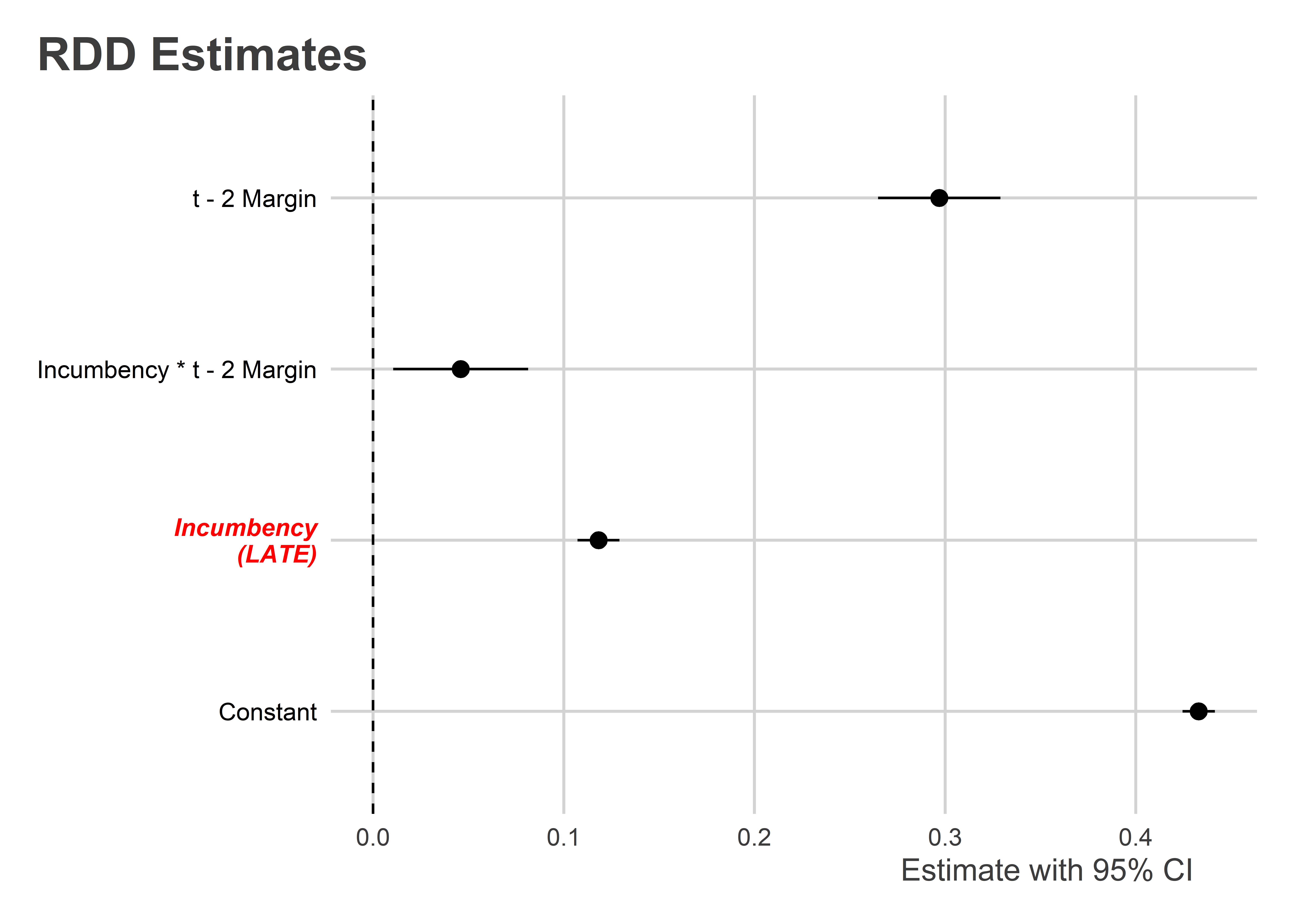
Seeing the data like this is useful, because it shows what this kind of interactive regression model is doing. However, just looking at the data doesn’t give us a firm estimate of the LATE. The below code shows how you can estimate the LATE using the lm_robust() function from {estimatr}. The results are visualized in a coefficient plot which shows the model estimate values with their robust 95% confidence intervals (x-axis) per each term in the model (y-axis).
## Add treatment column (1 = treated, 0 = otherwise)
house$tr <- (house$x>0)+0

## Estimate the model
rdd_fit <- lm_robust(
  y ~ tr * x,
  data = house,
  se_type = "stata"
)

## Show the results
tidy(rdd_fit) |>
  ggplot() +
  aes(
    x = estimate,
    xmin = conf.low,
    xmax = conf.high,
    y = term
  ) +
  geom_pointrange() +
  geom_vline(
    xintercept = 0,
    linetype = 2
  ) +
  scale_y_discrete(
    labels = c(
      "Constant",
      "Incumbency\n(LATE)",
      "Incumbency * t - 2 Margin",
      "t - 2 Margin"
    )
  ) +
  labs(
    x = "Estimate with 95% CI",
    y = NULL,
    title = "RDD Estimates"
  ) +
  theme(
    axis.text.y = element_text(
      color = c("black", "red", "black", "black"),
      face = c("plain", "bold.italic", "plain", "plain")
    )
  )
Instead of writing tr + x the above code is written as tr * x. This form tells R that it should estimate the interaction of the variables in addition to the lower order terms. For clarity, it tells R to estimate:
\[ \text{Vote Share}_{it+2} = \beta_0 + \overbrace{\beta_1 \text{Incumbent}_{it}}^\text{Lower order term} + \underbrace{\beta_2 \text{Vote Margin}_{it}}_\text{Lower order term} + \overbrace{\beta_3 \left(\text{Incumbent}_{it} \times \text{Vote Margin}_{it} \right)}^\text{Second order term} + \epsilon_{it+2} \]
If we wanted to be more explicit about this, we could instead write the formula in R like so:
lm_robust(y ~ tr + x + tr:x, data = house)Going back to the results, our RDD estimate tells us that the LATE equals 0.118. That means that incumbency confers a 11.8 percentage point boost to electoral performance for candidates close to the 0 percentage point vote margin. This estimate is also statistically significant with a p-value less than 0.001, so we can reject the null hypothesis that the LATE is zero.
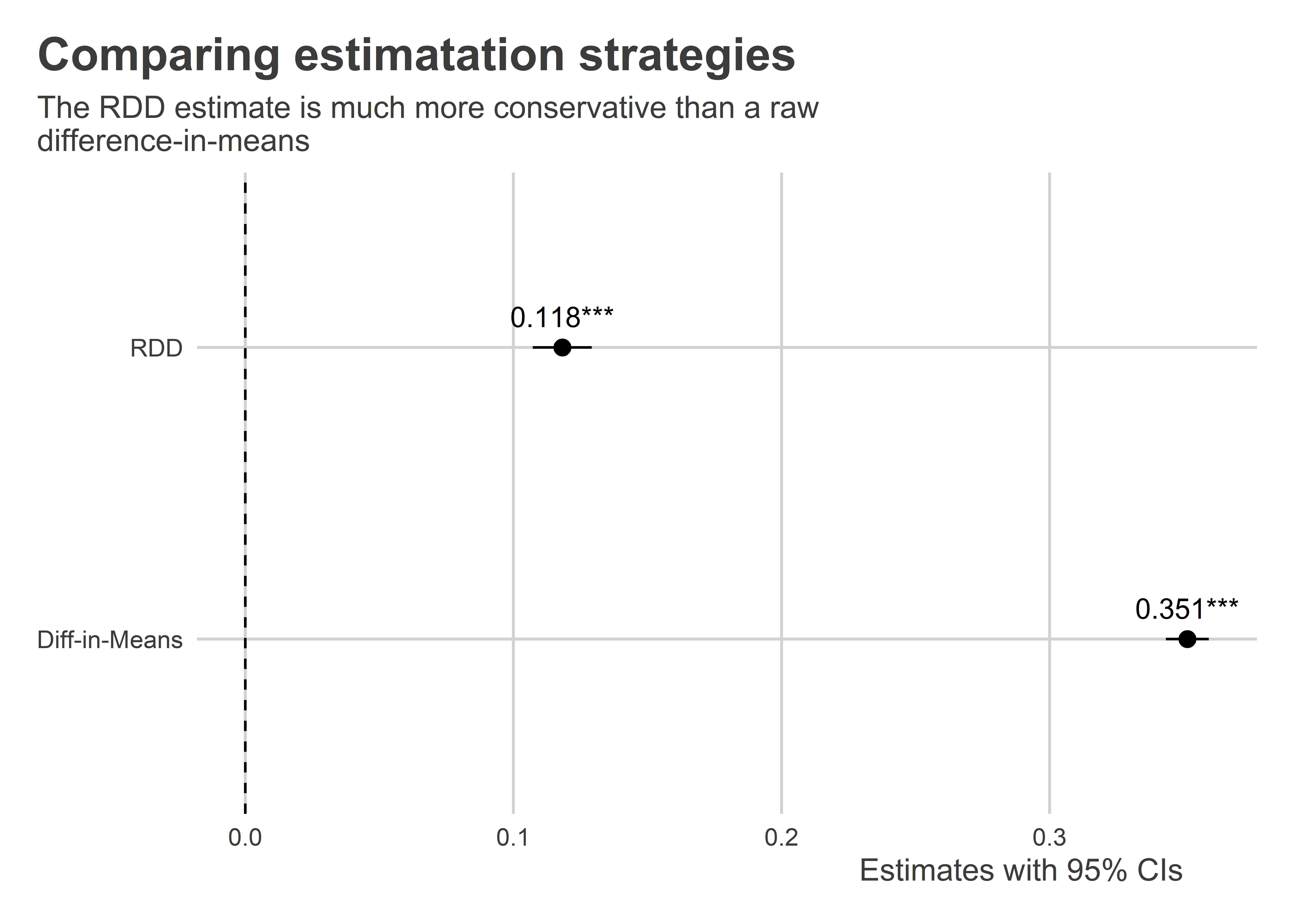
This is a much more conservative estimate of the incumbency effect that we’d get by taking a naive difference in means. We can compare the results of both approaches side-by-side:
## estimate simple diff-in-means
diff_fit <- lm_robust(y ~ tr, data = house, se_type = "stata")

## compare
bind_rows(
  tidy(rdd_fit),
  tidy(diff_fit)
) |>
  filter(
    term == "tr"
  ) |>
  mutate(
    model = c("RDD", "Diff-in-Means")
  ) |>
  ggplot() +
  aes(
    x = estimate,
    xmin = conf.low,
    xmax = conf.high,
    y = model
  ) +
  geom_pointrange() +
  geom_text(
    aes(
      label = paste0(
        round(estimate, 3),
        gtools::stars.pval(p.value)
      )
    ),
    vjust = -1
  ) +
  geom_vline(
    xintercept = 0,
    linetype = 2
  ) +
  labs(
    x = "Estimates with 95% CIs",
    y = NULL,
    title = "Comparing estimatation strategies",
    subtitle = "The RDD estimate is much more conservative than a raw\ndifference-in-means"
  )
14.3 Special considerations
The RDD approach to causal inference is a handy tool. But just like any tool, it should be used responsibly. So before you go out into the world thinking about how you can start applying the RDD willy nilly, there are some things you need to consider.
14.3.1 What are the counterfactuals in a RDD?
Underneath the RDD regression estimates are a set of implied counterfactuals. In particular:
library(geomtextpath)
ggplot() +
  geom_textline(
    data = house |> filter(tr==0),
    aes(x, predict(rdd_fit, house |> filter(tr==0))),
    label = "Observed non-incumbents"
  ) +
  geom_textline(
    data = house |> filter(tr==1),
    aes(x, predict(rdd_fit, house |> filter(tr==1))),
    label = "Observed Incumbents"
  ) +
  geom_textline(
    data = house |> filter(tr==0),
    aes(x, predict(rdd_fit, house |> filter(tr==0) |>
                     mutate(tr = 1))),
    label = "Unobserved non-incumbents",
    linetype = 2,
    color = "darkgray"
  ) +
  geom_textline(
    data = house |> filter(tr==1),
    aes(x, predict(rdd_fit, house |> filter(tr==1) |>
                     mutate(tr = 0))),
    label = "Unobserved Incumbents",
    linetype = 2,
    color = "darkgray"
  ) +
  labs(
    x = "Vote Margin",
    y = "Predicted Vote Share",
    title = "Implied counterfactuals in RDD"
  )
As you can see, the above shows that the treatment effect of incumbency is non-constant. This doesn’t really matter for the LATE we estimated, but it does matter for our ability to generalize beyond the point of the discontinuity. You should always be careful about interpreting the LATE and avoid making claims that go beyond what you can support with your data.
14.3.2 Bandwidth: Bias vs. precision
For many running variables, it is not always obvious how far out from the point of the discontinuity we should go when considering what observations to include in our analysis. In the U.S. House incumbency data we used all the data points, but that also means that the pre- and post-discontinuity slopes are influenced by observations that fall very far from the discontinuity itself. That can possibly bias our estimate of the LATE if these observations are really weird.
Therefore, sometimes we may think it’s a good idea to limit our “bandwidth” or “binwidth.” We may truncate our sample so that we drop observations beyond a certain distance from the discontinuity. Say we did so with the House data by only looking at margins +/- 25 percentage points from the incumbency threshold. Here’s what the data would look like:
ggplot(house) +
  aes(x = x,
      y = y) +
  geom_point(
    color = "gray"
  ) +
  geom_point(
    data = house |> filter(between(x, -0.5, 0.5)),
    color = "gray30"
  ) +
  geom_vline(
    xintercept = 0,
    lty = 2
  ) +
  geom_smooth(
    method = lm,
    aes(group = tr)
  ) +
  geom_smooth(
    method = lm,
    data = house |> filter(between(x, -0.5, 0.5)),
    aes(group = tr),
    color = "red"
  ) +
  labs(
    x = "Vote Margin in Last Election",
    y = "Vote Share",
    title = "Choice of bandwidth matters for RDD"
  )
Using the alternative bandwidth for the data, we get a slightly smaller estimate of the LATE:
rdd_fit2 <- lm_robust(
  y ~ tr * x, data = house |> filter(between(x, -0.5, 0.5))
)

## Show the results
## compare
bind_rows(
  tidy(rdd_fit),
  tidy(rdd_fit2)
) |>
  filter(
    term == "tr"
  ) |>
  mutate(
    model = c("With Full Data", "+/- 25 ppt")
  ) |>
  ggplot() +
  aes(
    x = estimate,
    xmin = conf.low,
    xmax = conf.high,
    y = model
  ) +
  geom_pointrange() +
  geom_text(
    aes(
      label = paste0(
        round(estimate, 3),
        gtools::stars.pval(p.value)
      )
    ),
    vjust = -1
  ) +
  geom_vline(
    xintercept = 0,
    linetype = 2
  ) +
  labs(
    x = "Estimates with 95% CIs",
    y = NULL,
    title = "Comparing estimatation strategies",
    subtitle = "The RDD estimate is much more conservative with a smaller\nbandwidth"
  )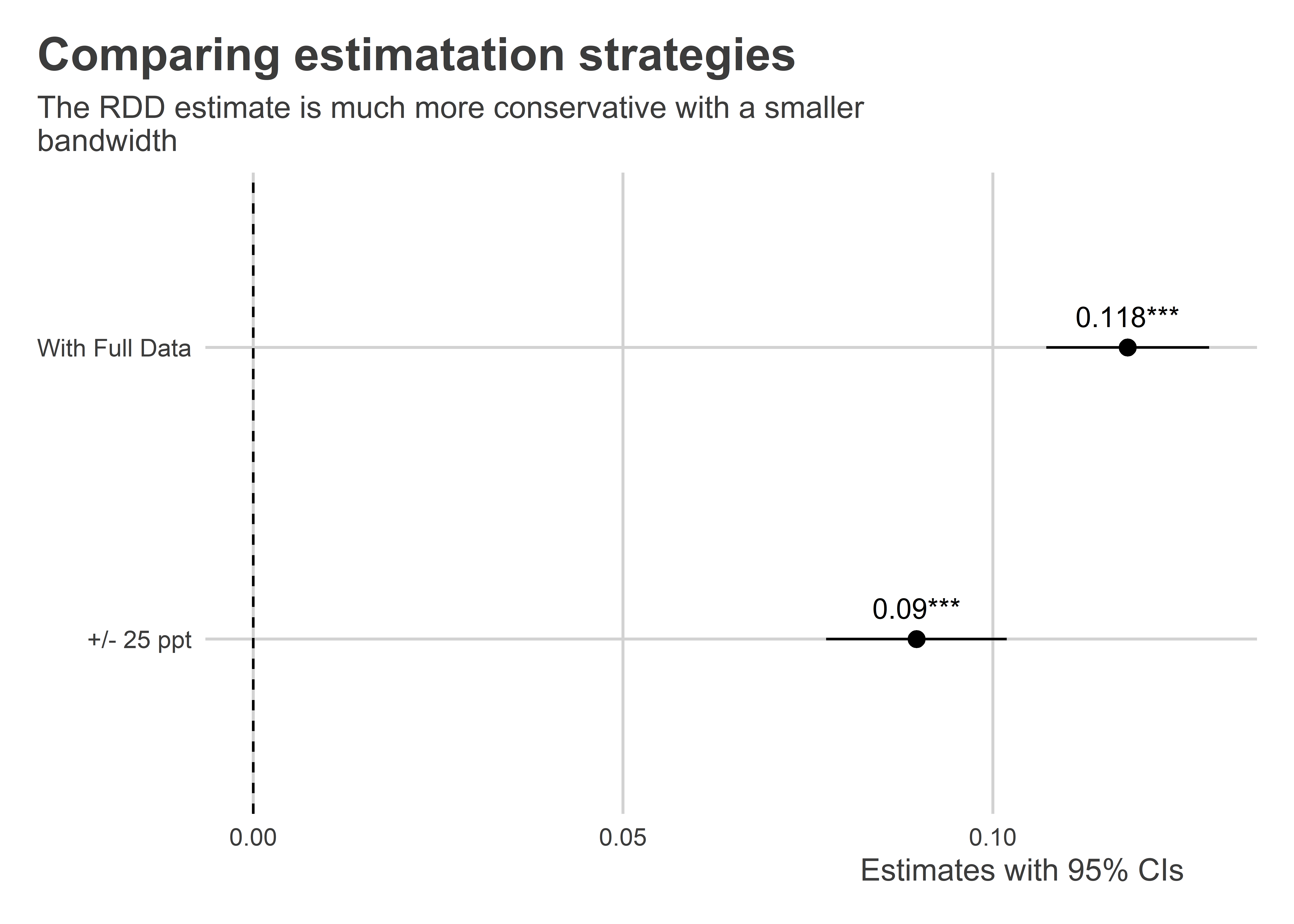
However, before you’re tempted to apply the most narrow bandwidth possible to the data, limiting the sample like this comes at a cost. Because we’re dropping data points from the analysis, we end up losing statistical precision. That means the narrower and narrower our bandwidth, the wider and wider our standard errors are going to get. The below code iterates over a bunch of different bandwidths and then plots the estimated LATE with its 95% CI:
# vector of binwidths:
bin_sizes <- seq(0.05, 1, by = 0.05)

# estimate the RDD for each binwidth:
bin_sizes |>
  map_dfr(
    ~ lm_robust(y ~ tr * x,
                data = house |>
                  filter(between(x, -.x, .x))) |>
      tidy() |>
      filter(term == "tr") |>
      mutate(
        bin = .x
      )
  ) -> results

# plot the results:
ggplot(results) +
  aes(x = bin,
      y = estimate,
      ymin = conf.low,
      ymax = conf.high) +
  geom_line() +
  geom_ribbon(
    alpha = 0.3
  ) +
  geom_hline(
    yintercept = 0,
    lty = 2
  ) +
  labs(
    x = "Bin size",
    y = "LATE with 95% CI",
    title = "The LATE using different bandwidths"
  ) +
  scale_y_continuous(
    labels = scales::percent
  )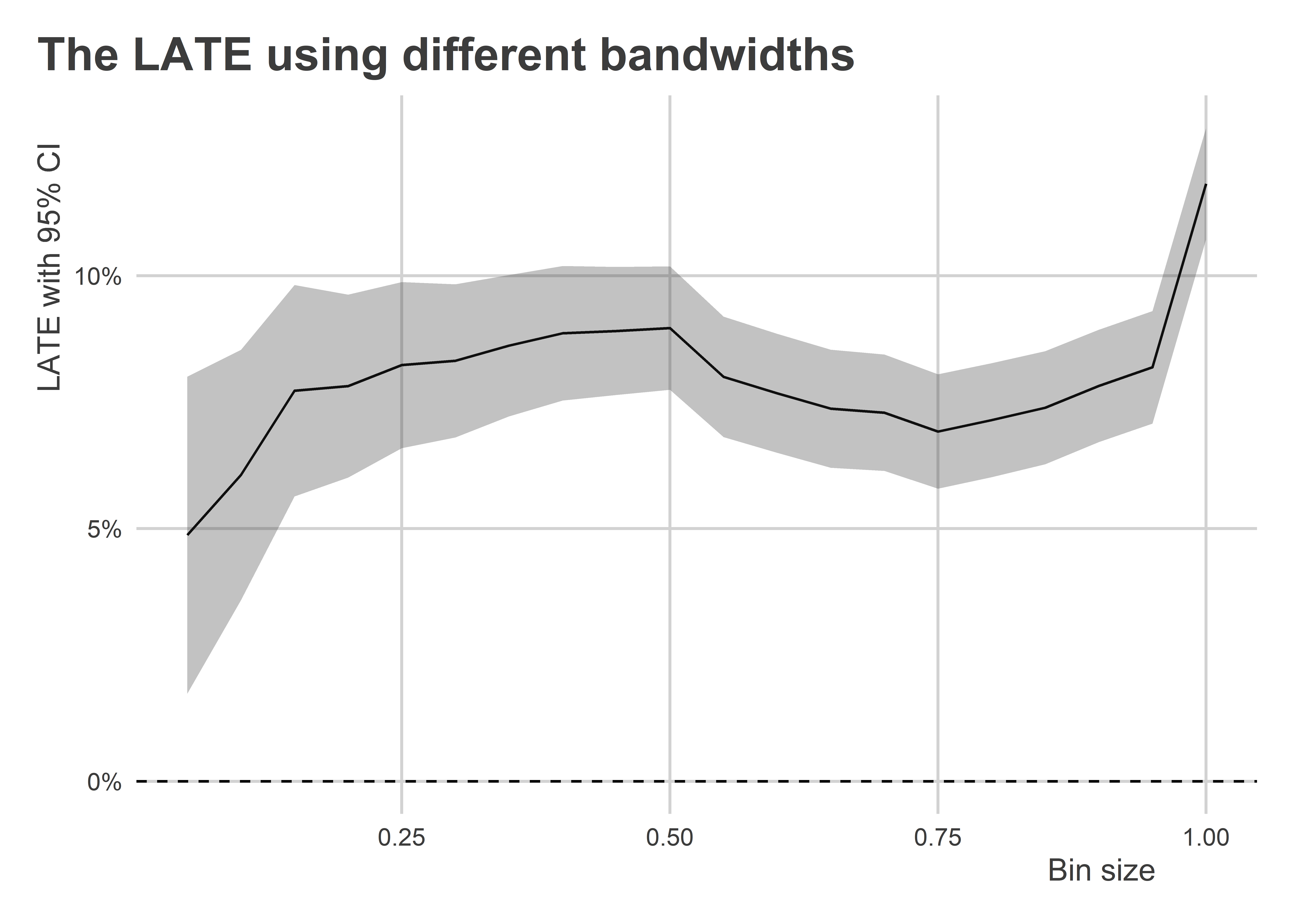
Clearly as we truncate the data closer to the point of the discontinuity, our estimate of the LATE of incumbency shrinks. When we get to a bandwidth of +/- 5 percentage points, the LATE is half the size of the original estimate we got using the full dataset. However, at the same time that narrowing the bandwidth attenuates the estimate of the LATE, it also leads to an inflation of our statistical uncertainty.
14.3.3 Continuity at the threshold
The validity of RDD hinges on the conceit that observations at the point of the discontinuity offer us apples-to-apples comparisons. This only works provided the discontinuity in the running variable doesn’t also influence other baseline characteristics of the units being studied.
In some real world cases, crossing the running variable threshold might be linked to a change in “treatment” status along a host of dimensions; not just one. That makes it hard to identify the causal effect of a single treatment since multiple things change about the status of observations at the point of discontinuity. Take the incumbency advantage. What exactly is this capturing? Do incumbents enjoy more financing? Do they have more experience? Do voters have a status quo bias? An RDD can’t tell us which factor is really the cause.
When you apply a RD design, you’ll need to do the work necessary to ensure continuity at the threshold plausibly holds. If it doesn’t, then you won’t be able to claim that you’re making apples-to-apples comparisons at the threshold.
14.3.4 Fuzzy RDDs
When we talked about randomized experiments, we discussed treatment compliance. Ideally, when individuals are assigned to treatment they will take the treatment. But that isn’t always the case. When it isn’t, just like we needed to take an instrumental variables approach in our experimental design, we need to do the same in our RD design.
When treatment is assigned perfectly at the discontinuity, we say we have a sharp RDD. But when it isn’t, say some people past the discontinuity aren’t treated and some before it are, we have a fuzzy RDD.
Let’s imagine a world where, somehow, third parties are more prevalent and competitive in US politics. They don’t dominate, but they’re prevalence is such that using the 0 margin threshold for congressional data no longer offers a sharp discontinuity in incumbency status. We can simulate this by randomizing the tr variable in the data for a narrow bandwidth of observations near the original discontinuity in the data:
house |>
  group_split(
    between(x, -0.1, 0.1)
  ) -> fuzzy_house
fuzzy_house[[2]]$tr <- sample(fuzzy_house[[2]]$tr)
fuzzy_house <- bind_rows(fuzzy_house)
Now, if we plot it:
ggplot(fuzzy_house) +
  aes(x = x,
      y = y,
      color = ifelse(tr==1, "Incumbent", "Not Incumbent")) +
  geom_point(
    alpha = 0.4
  ) +
  ggpal("binary") +
  geom_vline(
    xintercept = 0,
    lty = 2
  ) +
  labs(
    x = "Dem Vote Margin\n(Relative to Reps)",
    y = "Vote Share",
    color = NULL,
    title = "Fuzzy treatment assignment"
  )
We can clearly see that treatment is no longer perfectly determined by the running variable.
Here’s how we can recover an estimate of the LATE using a fuzzy RDD:
## Use iv_robust
fuzzy_fit <- iv_robust(
  y ~ tr * x | (x > 0) * x,
  data = fuzzy_house
)

## Check with "naive" sharp RDD
sharp_fit <- lm_robust(
  y ~ tr * x,
  data = fuzzy_house
)

## Compare
screenreg(
  list(fuzzy_fit, sharp_fit),
  include.ci = F,
  digits = 3
)
=======================================
             Model 1       Model 2
---------------------------------------
(Intercept)     0.376 ***     0.464 ***
               (0.007)       (0.004)
tr              0.223 ***     0.063 ***
               (0.012)       (0.006)
x               0.184 ***     0.366 ***
               (0.020)       (0.016)
tr:x            0.091 ***     0.013
               (0.019)       (0.018)
---------------------------------------
R^2             0.613         0.656
Adj. R^2        0.612         0.656
Num. obs.    6558          6558
RMSE            0.150         0.141
=======================================
*** p < 0.001; ** p < 0.01; * p < 0.05
You can see that using a standard regression approach yields a downward bias in the effect of incumbency.
The idea with the instrumental variables approach is to use the discontinuity threshold as the instrumental variable for the treatment. You then use the predicted likelihood of treatment as your causal variable rather than the treatment itself.
14.4 Conclusion
The RDD is a great tool of causal inference, and it has many advantages over the SOO design. However, to make it work, remember that you need a running variable that defines a threshold for or discontinuity in treatment assignment. This isn’t always the case. The next research design we’ll consider is very similar to this approach, but it is also more generalization to different contexts where a running variable isn’t available.