This chapter is best read in combination with “Chapter 4 - Correlation Requires Variation” in Thinking Clearly with Data (Bueno de Mesquita and Fowler 2021).
5.1 Learning Goals
Understand why variation is essential for learning about the correlation between two features of the world.
Understand what selecting on the dependent variable is and why it is not recommended for quantitative analysis.
Understand why the temptation/pressure to select on the DV persists.
5.2 Where we’ve been
We’ve been talking about correlation. Last time we introduced some important concepts related to correlation (mean, variance, covariance, linear regression, etc.) and discussed the utility of correlations (for description, prediction, and causal inference).
5.3 Where we’re going
I want us to sit with an important requirement for correlation: variation.
To estimate a correlation between two features of the world, we need variation in each of those features. This may seem obvious, but you’d be surprised by the number of real-world cases (in the media or even scholarly articles) where correlations or causation are inferred when at least one variable is missing variation.
In Chapter 2 of our Thinking Clearly with Data text, we saw a few examples of facts or descriptions about the world, some of which are correlations and others of which are not. Can you remember which are which?
People who live to 100 years of age typically take vitamins.
Cities with more crime tend to higher more police officers.
Successful people have spent at least 10,000 hours honing their craft.
Most politicians facing a scandal win reelection.
Older people vote more than younger people.
2 and 5 are the only two statements above that tell us about a correlation. 1, 3, and 4 sound like they tell us something about the relationship between two features of the world, but in reality they are missing variation in one of those features.
Take 1. The below R code simulates some data based on the kind of variation (or lack thereof) that statement 1 gives us. Can you catch the problem?
## open the {tidyverse}library(tidyverse) ## simulate some datavitamin_data <-tibble(live_to_100 ="Yes",take_vitamins =rbinom(n =200, size =1, prob =0.75)) ## plot the relationshipvitamin_data |>group_by(live_to_100) |>summarize(mean =mean(take_vitamins) ) |>ggplot() +aes(x = live_to_100, y = mean) +geom_col(width =0.5) +scale_y_continuous(labels = scales::percent ) +labs(x ="Live to 100?",y ="% who take vitamins" )
The problem is obvious. We don’t have variation in age!
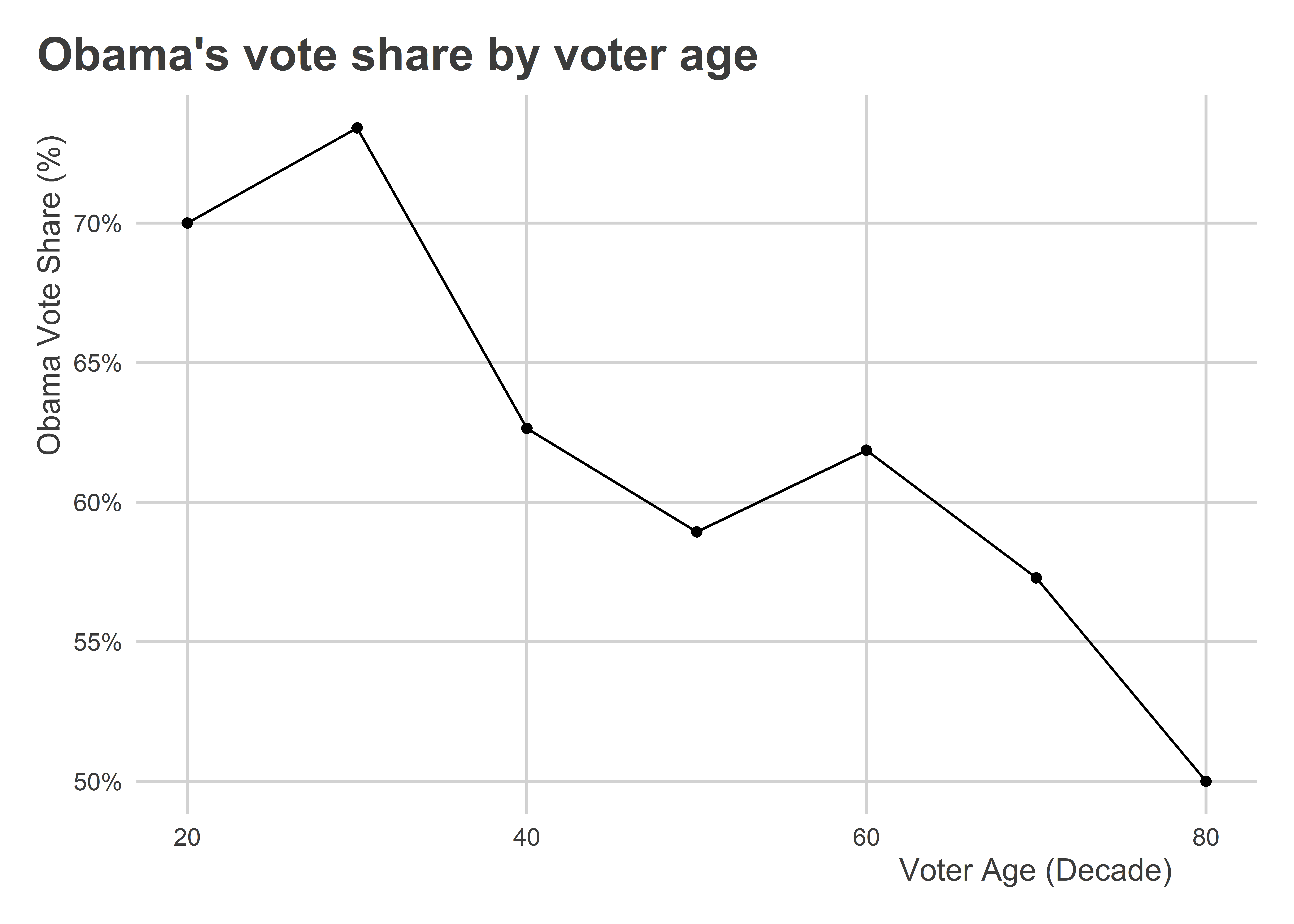
How about 5? Or something close to it anyway. In the below code, I’m attaching the {socviz} package which lets me access a dataset called gss_sm. This is a selection of individual responses to the 2016 General Social Survey. It has a variable for age and a variable for whether a person voted for Barack Obama in the 2012 election. Let’s check out their relationship.
library(socviz)## opening socviz to access gss_smlibrary(coolorrr)set_theme()## opening {coolorrr} to use the default theme with set_theme()## Make the data viz:gss_sm |>mutate(decade =floor(age /10) *10 ) |>group_by(decade) |>summarize(obama_vote =mean(obama, na.rm = T) ) |>drop_na() |>ggplot() +aes(x = decade, y = obama_vote) +geom_point() +geom_line() +scale_y_continuous(labels = scales::percent ) +labs(x ="Voter Age (Decade)",y ="Obama Vote Share (%)",title ="Obama's vote share by voter age" )
Can you identify a relationship? Of course you can! That’s because we have variation in both of these features of the world. We have some people who are older, some younger. And among those groups we have people who voted for Obama in 2012 and others that didn’t.
This analysis tells us something about a relationship or regularity in the world. The first, dealing with longevity and vitamins, does not. The fact that people who live to 100 years of age regularly take vitamins does not tell us whether taking vitamins actually promotes longevity. It’s just a bit of trivia about a particular age group.
5.4 Selecting on the DV
The mistake made in statement 1 is an example of selecting on the dependent variable (DV). Why would someone do this?
It’s actually easier than you many think to select on the DV, even without noticing. After all, the statement that “people who live to be 100 typically take vitamins” sounds scientific. But when we make things a little more explicit (like I did with the R code example above), it’s plain to see that this statement doesn’t actually tell us anything useful (certainly not actionable).
A lot of people slip into selecting on the DV when trying to make correlational (even causal) claims. This is partly a handicap of talking about these things in plain English. I have to admit, I had to think carefully about claims 1-5 above before I knew with certainty which dealt with correlations and which didn’t.
As pointed out in Thinking Clearly with Data, organizational/structural pressures may force researchers into selecting on the DV as well. Take the 2012 Republican party which did an “autopsy” after Romney lost the U.S. Presidential election. The autopsy-style of analysis is a prime example of selecting on the DV but one nonetheless that many political parties or corporations are tempted to do.
The dead give-away that a claim or analysis is predicated on selecting on the DV is that it starts with some phenomenon or outcome and then tries to look backward to identify causes. This is the case with the claim about vitamins and longevity. It starts with an outcome (living to over 100 years of age) and looks back at habits or lifestyle factors that are common to people who live to be this old.
We see a few different examples of this error in practice in Thinking Clearly with Data.
Malcom Gladwell’s claim that 10,000 hours of practice leads to becoming a great achiever.
Rock’n Roll is corrupting the youth.
High school dropouts.
Suicide attacks.
Let’s take a look at an example using some data that were collected in a 1998 field experiment involving a get out the vote (GOTV) campaign in New Haven, CT.
This dataset is in tidy format. It has 9 columns each corresponding to a different variable measured on individuals (the unit of observation). These variables are:
female: 0 = no, 1 = yes
age: in years
white: 0 = no, 1 = yes
black: 0 = no, 1 = yes
employed: 0 = no, 1 = yes
urban: 0 = no, 1 = yes
treatmentattempt: 0 = did not receive a GOTV phone call, 1 = did
successfultreatment: 0 = was not treated or didn’t answer the phone, 1 = answered the phone if treated
turnout: 0 = didn’t vote, 1 = did vote
For the sake of argument, let’s just look at folks who turned out to vote:
Data_turnout <- Data |>filter(turnout ==1)
With this filtered data, do you think we can figure out if getting a call increased turnout? Let’s see:
About 53-54 percent of people who turned out to vote received a GOTV phone call. 44 percent answered the phone. Did getting a call lead to an increase in the likelihood of turnout? What if we just look at the answer rate among phone call recipients?
82 percent of people who turned out to vote picked up the phone when they got a GOTV phone call. Does this tell us anything? It does in a sense. But does this say anything about the effect of calls on turnout? Not at all.
Without variation in turnout, we can’t say anything causal, let alone correlational.
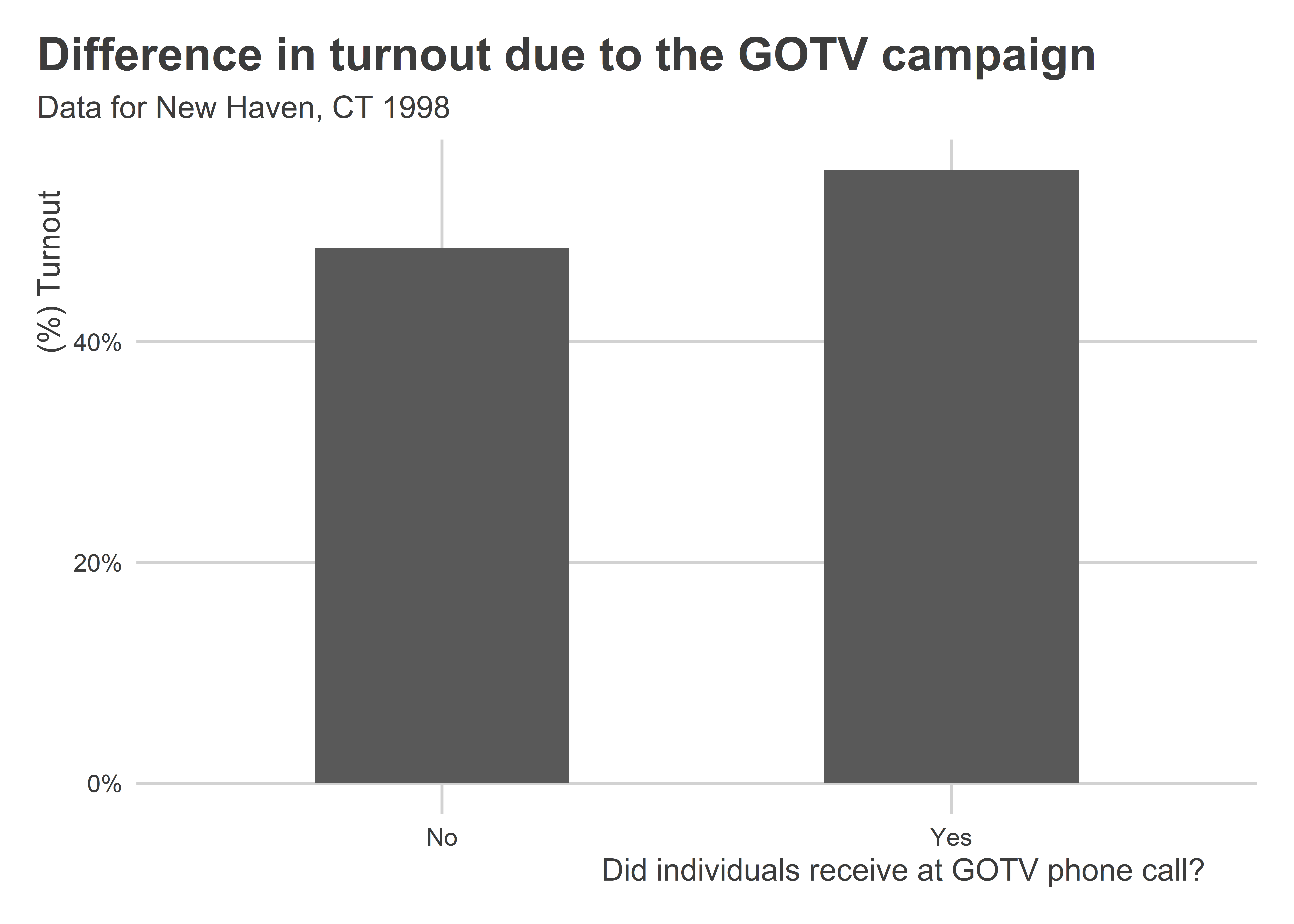
If we use the full dataset, we can start to draw some more informative conclusions. Below is some code that helps us answer this very question.
Data |>group_by(treatmentattempt) |>summarize(mean =mean(turnout, na.rm=T)) |>ungroup() |>mutate(xvar =ifelse(treatmentattempt==1, "Yes", "No")) |>ggplot() +aes(x = xvar,y = mean) +geom_col(width =0.5) +labs(x ="Did individuals receive at GOTV phone call?",y ="(%) Turnout",title ="Difference in turnout due to the GOTV campaign",subtitle ="Data for New Haven, CT 1998" ) +scale_y_continuous(labels = scales::percent )
When we look at the data we can clearly see a positive correlation between GOTV phone calls and turnout.
Can we make any causal claims? As it turns out, we don’t quite have enough basis for saying phone calls caused greater turnout. The data used for this analysis is infamous in political science because something went wrong with the field experiment. Households that received calls have some different characteristics compared to those that didn’t, and some of these characteristics might also explain higher turnout. This problem is called confounding, which we will return to later in this course.
Confounding aside, it is a fact that phone calls and turnout have a positive correlation. This can only be identified when we have variation in both turnout and whether individuals received a GOTV phone call.
5.5 “Proving” why we need correlation
It seems pretty obvious that there is no correlation without causation. Just to beat a dead horse, we can actually show mathematically that we need variation by seeing what happens when we try to estimate a correlation after selecting on the DV.
First, check out what happens when we use cor() with turnout and treatmentattempt from the Data_turnout dataset. We get an NA value returned.
Let’s consider the numerator of this equation first. What do you think the covariance between some variable is going to be if there is no variance in one of those variables? The below code calculates the covariance of turnout and treatmentattempt and saves it as an object called the_cov. It then tells R to report the contents. No surprise, the covariance is zero.
## estimate the covariancethe_cov <-cov( Data_turnout$treatmentattempt, Data_turnout$turnout)## report the resultthe_cov
[1] 0
Right off the bat, we can see that we’re not going to get either a positive or negative correlation for the variables of interest. But zero is still a meaningful correlation value—a zero means there is no linear relationship between two variables. Doesn’t this mean that a correlation is defined for our data?
Don’t forget that we still need to deal with the denominator in our correlation equation. To calculate a correlation, after we get the covariance for our variables of interest we need to divide them by the product of the standard deviations of each variable. The below code calculates the standard deviation of treatmentattempt and turnout and saves them as objects called sdx and sdy. It then reports the results. While treatmentattempt does have a non-zero standard deviation, turnout does not. You can only have a non-zero standard deviation if there is variation. No variation, no standard deviation.
sdx <-sd(Data_turnout$treatmentattempt)sdy <-sd(Data_turnout$turnout)## check them outsdx; sdy
[1] 0.4986888
[1] 0
Now, if you take some value and multiply it by zero, what do you get? You get zero:
sdx * sdy
[1] 0
And if you divide some value by zero, what do you get? You get an undefined value (that’s NaN in R-speak, which is short for “not a number”).
the_cov / (sdx * sdy)
[1] NaN
5.6 Wrapping up
By now, you should understand that to identify a correlation between two features of the world, you need variation in both of those features. Nonetheless, out of ignorance or organizational demands, researchers all-to-often select on the DV—they start with an outcome, look at other cases with the same outcome, and try to identify causes. This is a recipe for bad inference, and now you know why. Don’t forget this lesson, because recognizing when someone is making claims based on selecting on the DV can make you a better informed consumer of research.
5.7 Try out some examples yourself
Here are links to four different datasets that I simulated. For each one, there’s a research question. Get the data into R and see if it gives you the variation you need to answer the research question. If it can, answer the research question. If it can’t, can you leverage the data to draw inferences about other correlations? You’ll work in teams to find the answers.
Research Question: Do countries with higher GDP (gross domestic product) attract more immigrants?
Bueno de Mesquita, Ethan, and Anthony Fowler. 2021. Thinking Clearly with Data: A Guide to Quantitative Reasoning and Analysis. Princeton University Press.