7 Inference and Uncertainty

7.1 The Big Picture

All estimates are a function of signal, noise, and bias.
Because of noise and bias, our estimates contain an element of uncertainty.
With statistics, we can quantify this uncertainty, but we unfortunately cannot know how much bias is influencing our estimates.

7.2 Estimates, Populations, and Samples

Bueno de Mesquita and Fowler (2021) discuss a simple stylized formula for expressing where our estimates come from in data analysis. Specifically:

Estimate = Estimand + Bias + Noise

The values in this formula reflect different some different quantities of interest. Some of which we can measure and others of which we can’t:

Estimate: What we can actually calculate using our data.
Estimand: The true value we want to estimate but that we can’t ever observe.
Bias: Think of this as noise that systematically drives up or down our estimate. It becomes part of our estimate, but we can’t know for sure how big it is.
Noise: Random variation in the world that reduces our precision in estimating something of interest. We can summarize noise using statistics, but the estimate for noise will be a mix of some bias as well.

To get a sense for how these concepts work in practice, it is helpful to think in terms of populations and samples. This is the classical way to approach the question of uncertainty because the original purpose of statistics (why the mathematical field was created in the first place) was to say things about a broader population by looking only at a subset of it (sample). This is what pollsters do when trying to gauge support for the American President, for example.

The problem when making inferences about a population from a sample is that we always have uncertainty about the accuracy of our estimates. Except in the rarest of occasions, we never have all the data we need to calculate some relationship or characteristic of a whole population. That means we have no way to check that the relationship or characteristic that we observe in a sample matches the broader population. This is problematic, because our estimate of a relationship in, or characteristic of, a population could be influenced by bias or noise, or both.

Statistics doesn’t give us the ability to lift the veil on the capital “T” Truth, but it does give us the ability to precisely quantify our uncertainty. We can write some R code to demonstrate. Say the true share of people in a population of 1,000 who prefer Coke to Pepsi is 0.6. If we could ask all 1,000 people their preference, this is the value we’d calculate. This is called the estimand, and we’ll label it p. We can just assign an object called “p” in R the value 0.6.

p <- 0.6

Next, we can create our population of 1,000 and set it so that 60% of the population prefer Coke to Pepsi.

pop_size <- 1000
  # set the population size

population <- c(
  rep(0, (1 - p) * pop_size),
  rep(1, p * pop_size)
) # set it so p (0.6) share of the population like Coke
  # and the rest like Pepsi

If we were to take the mean of the population preferences, we would return 0.6:

mean(population)

[1] 0.6

A population of 1,000 is pretty small. It would probably be feasible to survey everyone about their soft drink preferences, but let’s say we’re under a limited budget and face a quickly approaching deadline. We only have the time and resources to ask 100 people.

Ideally, we would pick these 100 individuals at random to ensure that nothing will bias our estimate. We can use the sample() function to simulate the the random sampling process:

## use set.seed() to ensure replicability
set.seed(111)

## draw a random samaple and save it
the_sample <- sample(population, size = 100)

Now, instead of taking the mean of soda preferences with the population, we can instead do that with the sample:

mean(the_sample)

[1] 0.63

63% of people prefer Coke!

But wait…it should be 60% percent. What happened? Did we accidentally introduce bias? Quite the contrary. We randomly sampled individuals from the population. Instead, noise happened. The process of going from a population to a sample allows dumb luck creep into our estimate. If we kept repeating the sampling process, we would have some samples where we surveyed disproportionately more Coke-lovers, and others where we surveyed disproportionately more Pepsi-loves. It has nothing to do with systematic bias and everything to do with random chance.

The beauty of random sampling is that, on average, if we repeated the sampling process the mean of the sample estimates we calculate should closely approximate the population estimand. It would be impossible to do this in a real survey, but since this is a simulation, we can rerun the sampling process many times to confirm that random noise explains the differences we see and not bias.

Below, I use the map() function from the {purrr} package (part of the {tidyverse}) to iterate the sampling and estimation process. I then save the results as an object called sample_means. The nice thing about working with map() is that you can use it within the context of creating a new data frame. We can create a new data frame with the tibble() function. With it, I tell R that I want to make a data frame with a column called its (short for iterations) that takes all values from 1 to 1,000. I then add a second column called est that, for each iteration, reports a new sample mean. To do this, I give the map() function special instructions about the code it should rerun for each iteration using the code inside ~ { }.

## open {tidyverse} (also opens {purrr})
library(tidyverse)

## resample and estimate 1,000 times
times <- 1000

tibble(
  its = 1:times,
  est = map(
    its,
    ~ {
      new_sample <- sample(population, size = 100)
      new_mean   <- mean(new_sample)
      new_mean ## return the new mean
    }
  )
) |>
  unnest(est) -> sample_data

## look at the top 5 rows
sample_data |>
  slice_head(n = 5)

# A tibble: 5 × 2
    its   est
  <int> <dbl>
1     1  0.67
2     2  0.55
3     3  0.6 
4     4  0.59
5     5  0.61

We now have an empirical range of possible estimates. We can use a histogram to summarize the distribution.

## open {geomtextpath}
library(geomtextpath)

## make data viz
ggplot(sample_data) +
  aes(x = est) +
  geom_histogram(
    bins = 20,
    fill = "lightgrey",
    color = "darkgrey"
  ) +
  geom_textvline(
    xintercept = p,
    linewidth = 1,
    label = "The Population Mean",
    color = "darkblue"
  ) +
  geom_textvline(
    xintercept = mean(the_sample),
    linewidth = 1,
    linetype = 2,
    label = "Original Sample Mean",
    color = "darkred"
  ) +
  labs(
    x = "Range of Sample Estimates",
    y = "How Often They Occur",
    title = "Empirical Distribution of Sample Means"
  )

The range of estimates is wide. But, reassuringly, their central tendency lies around the true population mean.

When we account for this possible variation in the estimate due to sampling, we do so by calculating a margin of error. We can do this with what’s called a standard error. This is a lot like the standard deviation, but instead of summarizing how much data points in a sample diverge on average from the sample mean, it tells us how much our estimate of the mean diverges on average from the true population mean.

To see how these values are analogous, using these repeated sample estimates of the mean, we can calculate the standard error by simply taking the standard deviation of the set of sample means:

sample_data |>
  summarize(
    std_error = sd(est)
  )

# A tibble: 1 × 1
  std_error
      <dbl>
1    0.0463

Because we’re dealing with simulated data, it is easy enough to directly calculate the standard error. In practice, we usually can’t do this because we only have an estimate for one sample. So how do we compute the standard error? It turns out, via an approach that evokes an Inception-like, Leonardo DiCaprio-esque impression of events, we can repeatedly take samples from our sample to summarize our uncertainty about it.

We call this process bootstrapping, a term that supposedly dates back to the time of horses and muskets to describe a bizarre scenario where a soldier, he and his horse stuck in the mud, pulls himself and his horse out by pulling on his bootstraps. It’s utter nonsense, and the statistical procedure seems just as preposterous. But it works.

Here’s some code to make it happen. Just like before, I’m using a combo of tibble() and map(), but pay attention to what’s different this time:

tibble(
  its = 1:times,
  boot_est = map(
    its,
    ~ {
      ## calcuate sample size
      samp_size <- length(the_sample)
      
      ## bootstrap the sample
      re_sample <- sample(
        the_sample, 
        size = samp_size, 
        replace = T
      )
      
      ## estimate mean on bootstrapped data
      mean(re_sample)
    }
  )
) |>
  unnest(
    boot_est
  ) -> boot_data

## look at the first five rows
boot_data |>
  slice_head(n = 5)

# A tibble: 5 × 2
    its boot_est
  <int>    <dbl>
1     1     0.57
2     2     0.63
3     3     0.71
4     4     0.7 
5     5     0.59

Bootstrapping involves a simple process of resampling with replacement. The idea is to treat your sample like a stand-in population and repeatedly draw new samples from it. But there are two twists. The new samples will be the same size as the original. And, the samples will be drawn with replacement. That just means that every time an observation is drawn, it can also be drawn again. Generally a little over 62% of the new sample observations are unique. The rest might either be duplicates or triplicates of observations in the original sample.

We can check the distribution of these empirical bootstrap replicates using a histogram like before.

ggplot(boot_data) +
  aes(x = boot_est) +
  geom_histogram(
    bins = 20,
    fill = "lightgrey",
    color = "darkgrey"
  ) +
  geom_textvline(
    xintercept = 0.6,
    linewidth = 1,
    label = "The Population Mean",
    color = "darkblue"
  ) +
  geom_textvline(
    xintercept = mean(the_sample),
    linewidth = 1,
    linetype = 2,
    label = "Original Sample Mean",
    color = "darkred"
  ) +
  labs(
    x = "Range of Bootstrap Estimates",
    y = "How Often They Occur",
    title = "Empirical Distribution of Bootstrap Means"
  )

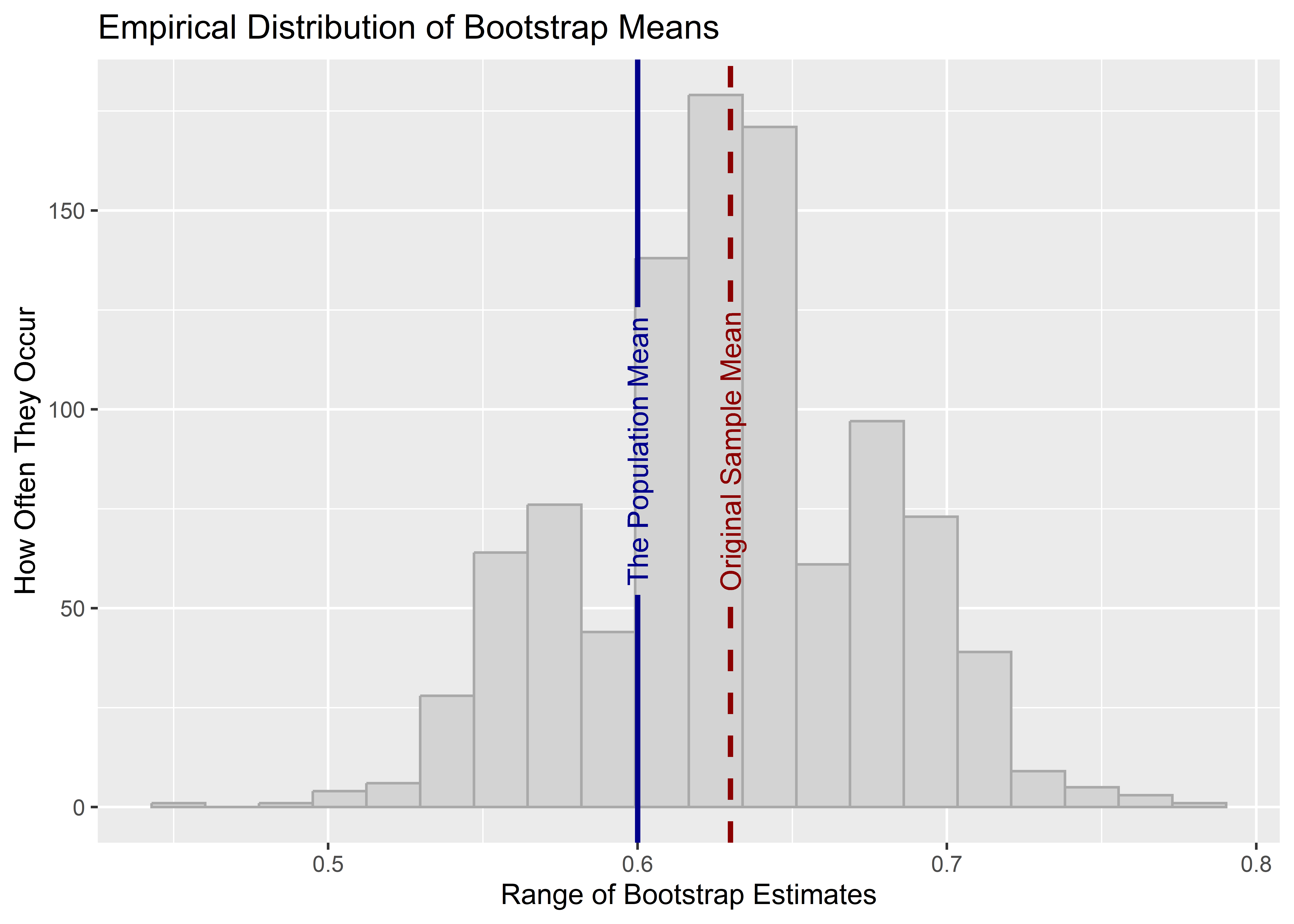
In this case, we can see that the true population mean is well within the range of the empirical bootstrapped distribution of estimates. But notice that the bootstrapped distribution is now centered on the original sample estimate of the mean rather than on the population mean. While the value around which the distribution is centered is not the same as with the population, the variance of the bootstrapped estimates should be about the same as the variance we got using the resampling procedure we used before. The code below reports the bootstrapped standard error and the resampling standard error side by side. Notice that while they are not identical, they are very similar.

full_join(
  sample_data,
  boot_data
) |>
  summarize(
    std_error = sd(est),
    boot_std_error = sd(boot_est)
  )

# A tibble: 1 × 2
  std_error boot_std_error
      <dbl>          <dbl>
1    0.0463         0.0479

7.3 Confidence Intervals and Hypothesis Testing

Generally, we don’t just calculate the standard error and leave it at that. We often use it to calculate 95% confidence intervals. Despite their less-than-helpful name, these intervals do not tell us how confident we are that a true population relationship or characteristic falls within said interval (they would if we were talking about Bayesian statistics, but that’s a subject for another day).

Instead, confidence intervals are just a way of summarizing uncertainty that is also helpful in hypothesis testing. We’ll go into more detail about hypothesis testing in the next chapter, but it’s helpful to introduce the concept here given its connection to uncertainty and confidence intervals. Specifically, confidence intervals give us a range around a sample estimate such that 95% of the time the true parameter would fall if we could take repeated samples and for each sample calculate another 95% confidence interval.

If that confuses you, just remember that:

Confidence intervals summarize uncertainty or imprecision in our estimate.
The wider they are, the more uncertainty or imprecision we have.
If they contain some value or reference point, we would say that our estimate is not statically different from that reference point at the 95% level. (This is the usual threshold for statistical significance in hypothesis testing.)

We can calculate these by multiplying the standard error by a constant. Bueno de Mesquita and Fowler (2021) say this value is 2, but it’s actually closer to 1.96. The code below calculates the upper and lower bound of the bootstrap based 95% confidence intervals for our sample estimate.

## calculate and save the sample estimate
sample_mean <- mean(the_sample)

## summarize values
boot_data |>
  summarize(
    sample_mean = sample_mean,
    boot_std_error = sd(boot_est),
    conf_lo = sample_mean - 1.96 * boot_std_error,
    conf_hi = sample_mean + 1.96 * boot_std_error
  )

# A tibble: 1 × 4
  sample_mean boot_std_error conf_lo conf_hi
        <dbl>          <dbl>   <dbl>   <dbl>
1        0.63         0.0479   0.536   0.724

Using this information we can test a hypothesis dealing with whether people in our population prefer one kind of soda for another. For hypothesis testing, we propose a null hypothesis and an alternative. The null is our point of reference and it holds that the true estimate of interest is zero or not different from some other value. In our soda example, the null would be that Coke is just as popular as Pepsi. An alternative hypothesis be that the population prefers Coke to Pepsi.

For any hypothesis we specify a level for our test. This is a threshold that we’ll use to determine whether we can reject the null hypothesis. By convention, we set the level to 5%. 95% confidence intervals, by extension, allow us to test against the null hypothesis using this test level. If the 95% confidence intervals don’t contain the value specified by the null hypothesis, then we can reject the null. Importantly, that doesn’t mean we can accept the alternative. As we’ll discuss more in the next chapter, we can only ever reject or fail to reject the null hypothesis. We never accept.

In the case of population preferences regarding soda, if we look at the 95% confidence intervals it is clear that we can reject the null hypothesis. How do we know? The lower bound of the 95% confidence intervals is greater than 0.5, which is the value we’d expect to see if the null hypothesis were true.

7.4 Calculating Uncertainty without Bootstrapping

The reason I showed you how to bootstrap above is not because that is the only way to calculate the standard error and, by extension, 95% confidence intervals. Instead, I showed you bootstrapping because I find it makes talking about standard errors much more intuitive. However, we can actually directly calculate the standard error using just our sample data itself, no resampling with replacement necessary.

For example, the equation for the standard error of the mean is just:

\[ \text{SE}_\mu = \frac{\sigma_x}{\sqrt{N}} \]

Remember that \(\sigma_x\) represents the standard deviation of some variable \(x\). To calculate the standard error, we just need to divided the standard deviation by the square root of the number of observations in the data. See the below code to check out how this approach compares to the resampling and bootstrapping approaches used above:

res_se <- sd(sample_data$est)
boot_se <- sd(boot_data$boot_est)
calc_se <- sd(the_sample) / sqrt(length(the_sample))

c(
  "Resampling" = res_se,
  "Bootstrapping" = boot_se,
  "Direct Calcuation" = calc_se
)

       Resampling     Bootstrapping Direct Calcuation 
       0.04631778        0.04789967        0.04852366

Notice that all three, while not identical, are very close in value.

If you’re paying attention, you might also notice that if the standard error is just the standard deviation divided by the sample size, then that means the bigger your sample the smaller the standard error. This makes sense, because the more data we have, the lower our uncertainty should be. Conversely, if we have only a small amount of data, our uncertainty about our estimate will be greater.

7.5 Be Careful of Bias

The process of quantifying uncertainty using standard errors and confidence intervals hinges on something really critical being true: no bias. Bootstrapping, for example, only works if the sample we’re bootstrapping from is a random sample. If the sample is biased in any way, it’s safe to say that our confidence intervals will mislead us because when we resample from a biased sample, we’ll get biased bootstrapped samples, too.

Unfortunately, unlike with noise, we have no way to quantify bias directly—unless of course we knew the “Truth.” This is why understanding, or better yet controlling, where your data come from is so essential to making sound inferences. The more you can do to ensure that the sampling process is random, the more you can be sure that bias is zero.

In the case of our data sample regarding soda preferences, we can feel confident that any deviations between the characteristics of the sample and the population result from random chance rather than a biased selection process. We could easily introduce some bias for illustration’s sake, however. Say that some unobserved characteristic, call it U, makes individuals harder to contact to ask them about their preferences. And, say Coke-lovers disproportionately have this characteristic. The below R code sets up the scenario.

# make population data
set.seed(111)
pop_data <- tibble(
  coke = population,
  u = rbinom(
    length(coke), 
    size = 1, 
    prob = 0.5 * coke + 0.25 * (1 - coke)
  )        # this bit here controls the prob of characteristic "u"
)

In our population of 1,000, Coke-lovers have characteristic U at twice the rate as Pepsi-lovers. By extension, that means Coke-lovers are about twice as unlikely to be contacted to ask them about their preferences. The below R code simulates how this affects the sampling process.

biased_sample <- pop_data |>
  # give the population data to slice_sample()
  slice_sample(
    n = 100, # pull out 100 observations
    weight_by = 1 - u # only picks non-U obs.
  )

Let’s check the sample mean to see if we notice anything odd.

mean(biased_sample$coke)

[1] 0.43

In the sample, only 43% of people indicated they prefer Coke to Pepsi. That’s way lower than in the actual population.

Even worse, if we calculated 95% confidence intervals for this sample, we’d find that our sample estimate is not statistically different from the population mean. Check it out:

biased_sample |>
  summarize(
    estimate = mean(coke),
    std_error = sd(coke) / sqrt(n()),
    conf_lo = estimate - 1.96 * std_error,
    conf_hi = estimate + 1.96 * std_error
  )

# A tibble: 1 × 4
  estimate std_error conf_lo conf_hi
     <dbl>     <dbl>   <dbl>   <dbl>
1     0.43    0.0498   0.332   0.528

Obviously with this biased sample our inferences are way off. Unfortunately, the tough thing about bias is that it’s difficult to devise a test to determine if it is present or influenced the collection or creation of our data. We know that the estimate shown above is influenced by bias only because we simulated the data. This is hard to do, often impossible, with real world data.

7.6 Inference and Forecasts

Not only can quantifying uncertainty help with making inferences about whether something is true in our population, we can also use statistical inference to summarize our uncertainty about our forecasts. For example, say we wanted to predict whether the sitting incumbent for US President, Joe Biden, will win the popular vote in the 2024 Presidential election. The below code reads in some data from all Presidential elections from 1948 to 2020. With that data, I tell R to estimate a linear forecast model of incumbent vote shares using an indicator of incumbent status, the incumbent party’s net approval rating, second quarter percent GDP growth, and an indicator for whether there’s a major third party candidate in the race.

## read in presidential forecast data
url <- "https://raw.githubusercontent.com/milesdwilliams15/Teaching/main/DPR%20201/Data/prez_data.csv"
prez_dt <- read_csv(url)

## fit a regression model to make predictions
prez_model <- lm(
  inc_vote ~ inc_running + inc_approval + 
    gdp_pct_growth + third_party,
  data = prez_dt
)

With this model, I can now generate a prediction for 2024. To do this, I first create a dataset using new values for the predictors in my model. Since Biden is the incumbent, I have that set to 1. For his net approval, I used his net approval according to Gallup as of the beginning of this year, taken as his approval minus disapproval rating. We don’t yet have second quarter GDP growth, so I did some sleuthing online and found some forecasts for the second quarter. They suggest it’ll be roughly 3%. I then assumed no major third party candidate would be involved. I then gave this data and my fit regression model to the predict() function. I also updated some settings. I selected se.fit = T and interval = "confidence" to tell predict to calculate a standard error for my prediction and then to use that to calculate a confidence interval. By default, it will return the 95% confidence interval. If you look at the output, it’s clear that 2024 is going to be a tight race. Biden is projected to get only slightly more than 50% of the vote. Even more, this prediction is not statistically different from the 50% point. In short, we have no basis for saying that Biden is statistically more likely to win the popular vote relative to the Republican challenger (who will probably be Trump).

## report prediction
new_data <- tibble(
  inc_running = 1,
  inc_approval = 0.41 - 0.54,
  gdp_pct_growth = 0.03,
  third_party = 0
)
predict(
  prez_model,
  newdata = new_data,
  se.fit = T,
  interval = "confidence"
) -> preds

## look at results
preds$fit

        fit       lwr       upr
1 0.5030413 0.4693492 0.5367333

Things would look worse if there were a third party challenger introduced to the race. Check out what this does to the prediction:

## report prediction
new_data <- tibble(
  inc_running = 1,
  inc_approval = 0.41 - 0.54,
  gdp_pct_growth = 0.03,
  third_party = 1
)
predict(
  prez_model,
  newdata = new_data,
  se.fit = T,
  interval = "confidence"
) -> preds

## look at results
preds$fit

        fit       lwr       upr
1 0.4304586 0.3961109 0.4648063

Not only is Biden projected to get nearly seven points below the 50% mark, this estimate is statistically different from 50% according to the 95% confidence intervals. This means that a third party challenger would be a major threat to Biden in 2024, making his projected performance statistically worse than his opponent’s.

7.7 What If My Sample Is the Population?

Our text covers this, but it’s worth carving out some space to think about this issue. You often see in research (mine included) individuals making statistical inferences when they have data for the full population under study. Why?

You’ll see a lot of explanations online, some better than others. My personal favorite is based on the multiverse (no, not the one from Marvel, though if you’re familiar you may get the idea). The idea is that reality contains an inherent randomness or, if you prefer, unknown sources of noise that could have resulted in any number of other observed relationships or outcomes in the world. That means any time we deal with a relationship between variables in a population, it could be the result of causation, or possibly just dumb luck. Some other unknown and unobserved variables in the population could explain it instead. We therefore would like to know the probability that the relationship we observe could have occurred due to pure chance.

The idea in more technical terms is that we assume our population data was produced from a data-generating process. It is therefore a sample of many possible datasets that could have been produced by this process. When this is the case, our goal is not to make inferences back to a population, it’s to make inferences about the data-generating process.

The takeaway is that, whether we have all the possible data points or only a sample, we still need to factor in uncertainty.

7.8 Conclusion

This is only the beginning of our exploration of statistical inference. Next time, we’ll talk more about hypothesis testing and the almighty p-value. The key things to remember are:

All estimates are a function of the truth, bias, and noise.
This means we need to use statistics to quantify the uncertainty associated with our estimates.
We can do this by calculating standard errors, which summarize how much our estimate is expected to deviate, on average, from the truth with repeated samples from a population or data-generating process.
One thing we can do with this summary of estimate uncertainty is to test hypotheses or claims about a broader population, or qualify the accuracy of our forecasts.